ISSN: 2374-2348 (Print), 2374-2356 (Online) Copyright © The Author(s). 2014. All Rights Reserved. Published by American Research Institute for Policy Development DOI: 10.15640/arms.v2n2a5 URL: http://dx.doi.org/10.15640/arms.v2n2a5
Restructuring Debt Model with Equivalent Equations: Theoretical and Practical Implications
Arturo García-Santillán1, Francisco Venegas-Martínez2 & Milka Elena Escalera-C hávez3
Abstract
This paper is aimed at developing a restructuring debt model between debtor and creditor. To do this, we use several hypothetic scenarios with some expired promissory notes and other documents which are not yet expired. The proposed equivalent equation model is useful to examine the three moments of the restructuring: valuing of the original debt, determining the new payment scheme, and computing new payments.
Keywords and Phrases: Restructuring debt, Equivalent equation, Promissory notes AMS Subjet Clasiffication: 62P05, 97M30
1.Introduction
The debt restructuring between debtors and creditors (clients, suppliers, companies) may sometimes be not so fair for one of the parties. That is, when there is no enough money to pay a previously acquired debt with some supplier of goods and/or services, it may be present an insolvency situation of the debtor for the payment of his/her obligation ([1, 3, 4]). This is very common when the cash flows have not been correctly budgeted, which could result in a payment default. In most cases, each promissory note which is due (owed), bring with it a small lapse of extension of time for delay.
1
ProfessorResearcher at Universidad Cristóbal Colón, Veracruz México and Posdoctoral ResearchFellow at EscuelaSuperior de Economía-IPN México. Email: [email protected]
2
Escuela Superior de Economía, Instituto Politécnico Nacional (ESE-IPN) México. Email: [email protected]
3ProfessorResearcher atUniversidad Autónoma de San Luis Potosí, SLP México, Posdoctoral ResearchFellow at
We are concerned, in this research, with developing a mathematical model that makes possible establishing a restructuring debt scheme between debtor and creditor resulting both benefitted. In this regard, García-Santillán and Vega-Lebrúm [4] suggested a scheme to establish a debt restructuring by a new payment schedule that best fits the needs of the debtor, provided that the creditor agrees. Both parts (debtor and creditor) should arrive at a consensus, in which everyone should be benefited from this agreement.
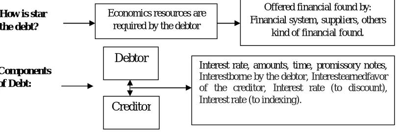
Regarding this, we answer the following question: Is there a model that allows calculate a debt restructuring in a way equitably for both parties? The variables of this study are displayed in Figure 1.
Figure 1: Component of Restructuring Debt (Adapted from García-Santillán and Vega-Lebrúm, 2008)
Right after obtaining any kind of credit, the credit immediately becomes a debt to whom receives the resource, beginning with this fact the relationship between the debtor and the creditor. We start the modeling with equivalent equations under the assumption that the debtor does not have to pay o the credit granted by the creditor [4, 5, 7]. In this regard, for instance, Citibank [8] raises a number of considerations which are associated with restructuring debt. First, we suppose that there are not problems of nonperforming loans. There are, of course, other factors which may be associated with the problem of debt default, for instance, financial crises.
Budgeting is a recommended practice because it is a tool which helps to organize and control flows, as indicated by Citibank [8].
Components of Debt:
How is star the debt?
Debtor
Creditor
Interest rate, amounts, time, promissory notes,
Interestborne by the debtor, Interestearnedfavor of the creditor, Interest rate (to discount), Interest rate (to indexing).
Economics resources are required by the debtor
Offered financial found by: Financial system, suppliers, others
It is clear that budgeting will not help to get out of debt; however, it will help to identify those expenses which are not necessary to get a reserve of money to amortize debt. It is always more advisable to seek a renegotiation or restructuring before a moratorium, suspension of payments, or bankruptcy declaration [4]. Citibank refers to this textually:
Definition 1. Negotiate with your creditor: "Do not fear to negotiate with
your creditor to devise a way to pay your debt: Design a plan to be presented to your creditors. It is recommended to pay the same amount each period to each creditor, or paying a little more to the creditor that charges the higher interest rate" [8].
From the above considerations, we develop a model that allow us to compute an equitable debt restructuring by using equivalent equations.
Scenarios to model:
a) Equivalent equations
Next, we will calculate a new payment scheme with equal payments through equivalent equations. From now on, we will denote the payment for each period by X. For the sake of simplicity, X takes the constant value of 1[2, 3, 6]. Once we get the value of VOD (valuation of original debt) and VNS (valuation of new scheme), we use them to get value of each equal payment (Y ) provided the payments have been agreed. If it is not the case, the new payments are calculated based on the agreed values, and the approach is different.
1.1 A formula for Restructuring Debt with Equivalent Equations
As usual, the formula that allows us to value the original debt with compounded interest rate is as follows:
1 . . .
1 1
1 . . .
1 2
/ /
1 . .
/
/ /
1 . .
/
( 1 ) ( 1 ) . . .
. . . D ( 1 ) . . .
( 1 ) ( 1 )
. . .
( 1 )
b f d n
b f d n n
n D
t m t m
i n d x i n d x
O D b f d b f d
n
D
a f d a f d
t m i n d x
b f d f d
t m t m
d d
n
a f d t m d
i i
V D D
m m
D D
i
D
m i i
m m
D i
m
After this, we calculate a new scheme with the next formula: 1... 1 1 1... 1 2 / / 1.. / / / 1.. /
(1
)
(1
)
...
...X
(1
)
...
(1
)
(1
)
...
(1
)
bfd n bfd n n n Dt m t m
indx indx
NS bfd bfd
n D afd afd t m indx bfd fd
t m t m
d d n afd t m d
i
i
V
X
X
m
m
X
X
i
X
m
i
i
m
m
X
i
m
In all cases X corresponds to each one of the payments. The resulting formula is:
1... 1 1 1... 1 2 / / 1.. / / / 1.. /
1
(1
)
1
(1
)
...
1
1
...1
(1
)
1
...
(1
)
(1
)
1
...
(1
)
bfd n bfd n n n Dt m t m
indx indx
NS bfd bfd
n D afd afd t m indx bfd fd
t m t m
d d n afd t m d
i
i
V
m
m
i
m
i
i
m
m
i
m
Finally, in order to obtain the each equal payment value, we use
Where:
debr=debtor crtr= creditor n = time (∑t/m) m = capitalization
Ip = Interestborne by the debtor
Ig = Interestearnedfavor of the creditor
id/m =Accurate Interest rate (to discount)
(∑id/365*m)
iindx/m =Accurate Interest rate (to indexing)
(∑iindx/365*m)
fd= focal date afd= after focal date bfd= before focal date D1, ….Dn= Document1,
…Documentn(promissory notes)
VOD= Valuation original debt
VNSP= Valuation new scheme of
payments Y= equal payment
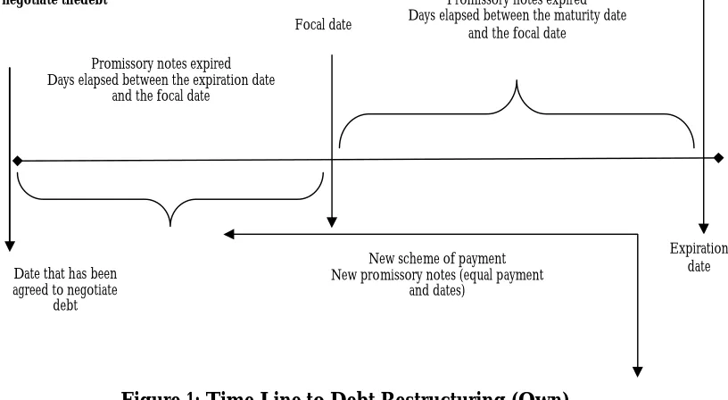
In order to have an illustrative approach to the model, we provide Figure 2, in which the line of time shows the moment when the debt restructuring is established.
Figure 1: Time Line to Debt Restructuring (Own)
If we are unable to pay some promissory notes, considering that some of these have already been expired (they have not paid), then the negotiation begins. The focal date is set, the original debt is valued, i.e., the expired promissory notes are valued (indexed), and the promissory notes not expired are valued too. The latter are brought to present value to the focal date by using a discount factor. Subsequently, the new payment schedule is established.
Date that has been agreed to negotiate
debt
Expiration date Promissory notes expired
Days elapsed between the maturity date and the focal date
Focal date
Agreed to negotiate thedebt
Promissory notes expired Days elapsed between the expiration date
and the focal date
New scheme of payment New promissory notes (equal payment
It is therefore necessary to calculate the coefficient of payments which is required for the denominator of the formula Y = VDO=VNE.
Hence, it is important to be aware that the factors for accumulation and discount, and it will be required to have the nominal rate that will become effective for the valuation of the expired promissory notes (the highest rate) and the real interest rate (the lowest rate) for the discounting of not expired promissory notes.
2. Methodology
2.1 Debt Restructuring with Equivalent Equations
In order to compute variable Y (amount of each payment) in a debt restructuring between debtor and creditor, we use hypothetic scenarios with some expired promissory notes and other promissory notes that are not yet expired. Therefore, we will be using an equivalent equation model to calculate the three moments of the restructuring: valuation of the original debt (VOD), valuation of the new payment scheme (VNSP) and calculate the amount of each new payments (Y).
Moreover, for indexation of all promissory notes which have been expired, we will use the effective interest rate; otherwise, to discount the value for all promissory notes not expired, we utilized the real interest rate.
where:
TN=Nominal interest rate for indexing 12 % (should become to effective interest rate),
TR=Nominal interest rate for discounting = unknown (the real interest rate) TI=Inflation rate 3.5%
2.1.1. Time line path in Restructuring
2.1.2. Data for Development an Equivalent Equation Model
Promissory notes
Due date (expired or maturity)
id = Accurate
Real Interest rate (to discount)
iindx =
Accurate Effective Interest rate (to indexing) Amount (Thousands of dls.)
DATA: Nominal exchange rate 12%, Inflation rate 3.45%, capitalization every 27 days (for all cases), effective interest rate and real interest rate are unknown?
F1 Expired 171
days ago (bfd)
(∑iindx/365*m) $100.00 In order to calculate the three
moment in debt restructuring (VOD, VNS and Y), we determine:
1.- For VOD (valuation original
debt)
a.-utilize effective interest rate for all document expired (bfd)
/ )n m 1
i m
Te = (1+ *100
b.- utilize real interest rate for all document not expired (afd)
( )
(1
T e T I T I
T R = * 10 0
2.- For VNSP (valuation new
scheme of payment) a.-utilize real
interest rate for all new scheme of payment: before focal date and after focal date
( ) (1 Te TI TI
TR = *100
F2 Expired 163
days ago(bfd)
(∑iindx/365*m) $120.00
F3 Expired 78
days ago(bfd)
(∑iindx/365*m) $115.00
F4 Expired 35
days ago(bfd)
(∑iindx/365*m) $90.00
F5 Expired in
focal date (fd) Without interest rate
$71.50
F6 Debt with a
maturity of 31 days (afd)
(∑id/365m) $111.00
F7 Debt with a
maturity of 67 days(afd)
(∑id/365*m) $123.00
F8 Debt with a
maturity of 81 days(afd)
(∑id/365*m) $200.00
F9 Debt with a
maturity of 131 days(afd)
(∑id/365*m) $300.00
F10 Debt with a
maturity of 171 days(afd)
(∑id/365*m) $190.00
Source: (provided by the authors)
F3bf
d
F2bf
d F5f
d F1bf d F4bfd Future time F6af d Pass time
2.1.3. The New Scheme of Equal Payments is as Follow
Promissory notes
Pn
D1, ….Dn= Document1,
…Documentn
Date
(before, in focal date or after)
Equal payment
Promissory notes Pn1 25.65 days before focal date
20 equal payments
OD NSP
V Y
V
Promissory notes Pn2 19.5 days before focal date
Promissory notes Pn3 7.87 days before focal date
Promissory notes Pn4 In the focal date focal date
Promissory notes Pn5 1.5 days after focal date
Promissory notesPn6 45 days after focal date
Promissory notesPn7 75 days after focal date
Promissory notesPn8 115 days after focal date
Promissory notesPn9 120 days after focal date
Promissory notesPn10 150 days after focal date
Promissory notesPn11 168 days after focal date
Promissory notesPn12 181 days after focal date
Promissory notesPn13 197 days after focal date
Promissory notesPn14 245 days after focal date
Promissory notesPn15 270 days after focal date
Promissory notesPn16 297 days after focal date
Promissory notesPn17 320 days after focal date
Promissory notesPn18 348.75 days after focal date
Promissory notesPn19 370.189 days after focal date
Promissory notesPn20 500 days after focal date
Source: (provided by the authors)
3. Theoretical and Empirical Results
OD
NSP
V
=
V
Y
3.1 Debt Restructuring
First, we calculate indexing and discounting factors for VOD (valuation of original debt)
1.- For indexing the effective interest rate is used for all expired promissory notes (bfd)
n/m
365/27
i
= (1+
)
-1 *100
m
.12*27
= (1+(
)
-1 *100
365
Te
13.5185185
= (1+ (0.00887671) -1 *100 = 1.126899997 -1 *100
= 12.6899997
Te
2.- For discounting the real interest rate is used for all not expired promissory notes (afd)
(T e - T I) (.1 2 6 8 9 9 9 9 7 - 0 .0 3 5 ) (.0 0 9 1 8 9 9 9 9 7 )
= * 1 0 0 = =
(1 + T I 1 .0 3 5 1 .0 3 5
T R
= 0.08879227 *100
= 8.879227
TR
Now, to calculate the valuation of new payment scheme (VNSP), we usethe
same factors asinVOD
1.- For indexing the effective interest rate is used for all new promissory notes that shall pay before focal date (bfd)
n/m
i
= (1+
)
-1 *100
m
Te
= 12.6899997
Te
2.- For discounting the real interest rate is used for all new promissory notes that shall pay after focal date (afd)
( T e - T I)
=
* 1 0 0
(1 + T I
= 8 .8 7 9 2 2 7
T R
T R
Finally, we calculate the interest rate capitalization every 27 days utilizing Teand TR as follow:
For VNSPall promissory notes that will pay before focal date
capitalization
.126899997 * 27
i
=
= 0.00938712
365
For VNSPall promissory notes that will pay after focal date
capitalization
.08879227 * 27
i = = 0.0065682
365
3.2 Valuation of Original Debt
1... 1 1 1... 1 2 / / 1.. / / / 1.. /
(1 ) (1 ) ...
...D (1 ) ...
(1 ) (1 )
... (1 ) bfd n afd n n n D
t m t m
indx indx
OD bfd bfd
n D afd afd t m indx bfd fd
t m t m
d d n afd t m d i i
V D D
m m
D D
i
D
m i i
m m D i m
b fd1...n A fd1...n D17 1/ 27 1 63 / 2 7
O D 1..n
78 / 27 35 / 27
D
31/ 27 1..n
V = $1 00 .0 0(1 + 0 .0 0 93 87 1 2) + $1 2 0.0 0 (1 + 0.00 93 8 71 2) + ... ... + $ 11 5 .0 0(1 + 0 .0 09 38 7 12 ) $9 0.00 (1 + 0 .00 9 3 8 71 2 ) + $ 71 .5 0 + ...
$1 11 .0 0 $ 12 3 .0 0 +
(1 + 0 .0 06 5 68 2) (1 + 0 .0 06 5 6
67 / 2 7 81/ 27131/ 27 17 1/ 27
$2 0 0.0 0
+ + ...
8 2) (1 + 0.00 65 6 82 ) $ 30 0 .0 0 $ 1 90 .0 0
... +
(1 + 0.00 6 56 82 ) (1 + 0 .00 6 56 82 ) bfd1...n Afd1...n D 6.3333333 6.03703704 OD 1..n 2.8888889 1.29629630 D 1.14814815 1..n
V = $100.00(1.00938712) + $120.00(1.00938712) + ...
... + $115.00(1.00938712) + $90.00(1.00938712) + $71.50 + ...
$111.00 $1
... +
(1.0065682)
2.48148148 3131/ 27 6.3333333
23.00 $200.00 + + ... (1.0065682) (1.0065682) $300.00 $190.00 ... + + (1.0065682) (1.0065682) bfd1...n Afd1...n D OD 1..n D 1..n
V = $100.00(1.06096031) + $120.00(1.05802722) + ...
... + $115.00(1.02735944) + $90.00(1.01218537) + $71.50 + ...
$111.00 $123.00 $200.00
... + + + ...
1...
1...
1.. 1..
$106.10 $126.96 $118.15 $91.1 $71.50 ...
... $110.17 121.02 196.11 290.62 182.28
$1,414.00
bfd n
afd n
D
OD n D
n
OD
V
V
In this way, we obtain the total value of original debt.
3.3 Valuation of the New Scheme of Payments
To assess the new scheme of payment, we use the indexation factor for all new payment before the focal date and to value all the new payment after the focal date we use the discount factor. It is also necessary utilize the interest rate with capitalization every 27 days, from the effective interest rate and real interest rate, respectively. After this, we assess a new scheme with the following formula:
1 ...
1 1
1 ...
1
2
/ /
1 ..
/
/ 1 ..
/ /
(1 ) (1 ) ...
... X (1 ) ...
(1 )
... ...
(1 ) (1 )
b f d n
a fd n
n
n
D
t m t m
i n d x in d x
N S P b fd b fd
n
D
a fd t m
i n d x
b f d fd
t m d
n
a f d a f d
t m t m
d d
i i
V X X
m m
X i
X
m i
m X
X
i i
m m
In all cases X = corresponding to each one of the payment
D
1...n
bfd i åt / m i åt / m
indx indx
VNSP = 1bfd (1 + m ) + 1bfd (1+ m ) ...
1..n 1 1
Dafd1...n 1afd
i åt / m 1
indx
...1 (1 + ) + 1 + + ...
m
bfdn fd 1..n id åt / m
(1+ )
m
1 1
afd2 afdn
...+ ...
i åt / m i åt / m
d d
(1 + ) (1 + )
m m
Thus, we have:
bfd 1...3
1 2
afd 1...16
5
3 4
6
D
25.65 / 27 19.5 / 27
NSP bfd bfd
1....16
D
afd 7.87 / 27
bfd fd 1.5 / 27
1...16
afd afd
45 / 27
V = 1 (1+ 0.00938712) + 1 (1+ 0.00938712) + ...
1
...+ 1 (1+ 0.00938712) + 1 + + ...
(1+ 0.0065682)
1 1
...+ +
(1+ 0.0065682)
...
7 8
9 10 11
13 14
12
afd
75 / 27 115 / 27
afd afd afd
120 / 27 150 / 27 168 / 27
afd afd
afd
181 / 27 197 / 27
1
+ + ...
(1+ 0.0065682) (1+ 0.0065682)
1 1 1
...+ + + + ...
(1+ 0.0065682) (1+ 0.0065682) (1+ 0.0065682)
1 1
1
+ +
(1+ 0.0065682) (1+ 0.0065682) (1+ 0.0
...
15 10 17
18 19 20
245 / 27
afd afd afd
270 / 27 297 / 27 320 / 27
afd afd afd
348.75 / 27 370.189 / 27 500 / 27
+ ... 065682)
1 1 1
...+ + + + ...
(1+ 0.0065682) (1+ 0.0065682) (1+ 0.0065682)
1 1 1
+ +
(1+ 0.0065682) (1+ 0.0065682) (1+ 0.0065682)
Now we have:
b fd 1 .. ... .3
1 2
a fd 1 .. ... 1 6
5
3 4
6 D
0 .9 5 0 0 0 0 0 0 .7 2 2 2 2 2 2
N S P b fd b fd
1 ...1 6
D
a fd 0 .2 9 1 4 8 1 5
b fd fd 0 .0 5 5 5 5 6
1 ...1 6
a fd a
1 .6 6 6 6 6 6 7
V = 1 (1 .0 0 9 3 8 7 1 2 ) + 1 (1 .0 0 9 3 8 7 1 2 ) + ... 1
...+ 1 (1 .0 0 9 3 8 7 1 2 ) + 1 + + ... (1 .0 0 6 5 6 8 2 )
1 1
...+ +
(1 .0 0 6 5 6 8 2 )
...
7 8
9 1 0 1 1
1 3 1 2
fd a fd
2 .7 7 7 7 7 7 8 4 .2 5 9 2 5 9 3
a fd a fd a fd
4 .4 4 4 4 4 4 4 5 .5 5 5 5 5 5 6 6 .2 2 2 2 2 2 2
a fd a
a fd
6 .7 0 3 7 0 3 7 7 .2 9 6 2 9 6 3
1
+ + ...
(1 .0 0 6 5 6 8 2 ) (1 .0 0 6 5 6 8 2 )
1 1 1
...+ + + + ...
(1 .0 0 6 5 6 8 2 ) (1 .0 0 6 5 6 8 2 ) (1 .0 0 6 5 6 8 2 )
1 1
1
+ +
(1 .0 0 6 5 6 8 2 ) (1 .0 0 6 5 6 8 2 )
...
1 4
1 5 1 0 1 7
1 8 1 9 2 0
fd
9 .0 7 4 0 7 4 1
a fd a fd a fd
1 0 .0 0 0 0 1 1 .0 0 0 0 0 1 1 .8 5 1 8 5 1 9
a fd a fd a fd
1 2 .9 1 6 6 6 6 7 1 3 .7 1 0 7 0 3 7 1 8 .5 1 8 5 1 8
+ ... (1 .0 0 6 5 6 8 2 )
1 1 1
...+ + + + ...
(1 .0 0 6 5 6 8 2 ) (1 .0 0 6 5 6 8 2 ) (1 .0 0 6 5 6 8 2 )
1 1 1
+ +
(1 .0 0 6 5 6 8 2 ) (1 .0 0 6 5 6 8 2 ) (1 .0 0 6 5 6 8 2 )
5
Moreover we have
bfd1...3
1 2 3
afd1...16
5 6 7
4
8 9
D
NSP bfd bfd bfd
1..3 D
afd afd afd
fd
1...16
afd afd
V
=
1 (1.00891568)+1 (1.00677078)+1 (1.00272712)+...
1
1
1
...+1 +
+
+
+...
(1.00036377) (1.01097095) (1.0183517)
1
1
...+
+
+
(1.02827659) (1.02952399)
...
10 1113 14 15
12
10 17 18 19
afd afd
afd afd afd
afd
afd afd afd afd
1
1
+
+...
(1.03704019) (1.04157623)
1
1
1
1
+
+
+
+...
(1.04486459) (1.04892605) (1.06120542) (1.06765775)
1
1
1
1
...+
+
+
+
(1.07467034) (1.08068035) (1.08824014) (1.093911
Therefore, we obtain the individual coefficients
bfd1...n3
afd1...16
D
NSP 1..3
D
1...16
V
=
1.00891568+1.00677078+1.00272712+1+...
...+
0.99963636+0.98914811+0.98197901+0.97250098+...
...+0.97132268+0.96428278+0.96008336+0.95706182+0.95335605+...
...+0.9423
2462+0.93662974+0.93051791+0.925343+0.91891482+...
...+0.91415039+0.88582522
Finally, in order to obtain the value of equal payment:
$1,414.00
19.2214904 $73.5634943
$73.56
Y
Y
Y
4 Conclusions
In the illustrative example that we set, the original debt was of $1,420.50. The new scheme of payment is $73.56 * 20 = $1,471.20 and the difference is $50.70, which is the dividend earned by the creditor. As we saw in this paper, a financial strategy that could favor an equitable settlement for all parties involved may be a debt restructuring models using equivalent equation.
Similarly, the debtor may have benefit at the moment to use the discount factor to reduce the future value of the debts that are not required. In this way, when we bring to the focal date all of the flows of indexed and discounted promissory notes that have been valued, then we find a fair balance between the apportionment of interest rates and times, which finally benefits both creditor and debtor.
Acknowledgements
The authors are very grateful to the anonymous referees for all suggestions, as well as Universidad Cristobal Colón in Veracruz and Escuela Superior de Economía del InstitutoPolitécnicoNacional for support. And very special thanks to Felipe de Jesús Pozos Texon, a Ph.D student in the doctoral program at UCC, for helping us to get the Latex format of this paper.
References
Ayres, Frank, 1991. Theory and Exercises of Financial Mathematics.McGraw-Hill.p. 230. Highland, E. H., 1987. Financial Mathematics.Prentice-Hall.pp 622-235
García-Santillán, A., 2011. Financial Management I. EuroMediterranean Network, Full text at: Universidad de Málaga, ISBN-13: 978-84-693-7162-6. Retrieved from:
http://www.eumed.net/libros/2010c/729/index.htm
García-Santillán, A., and Vega-Lebrúm, C. (2008): Debt restructuring through a common factor and equivalent equation modeling. Contributions to Economics, abril 2008. Moore, Justin H., 1963. Financial Mathematics.UTEHA. XV,
Portus, Govinden Lincoyan, 1997. Financial Mathematics.McGraw-Hill. Zima, Petr, 2005. Financial Mathematics.McGraw Hill.