*Corresponding author
Email address: [email protected]
1. Introduction
The increase produced in mobility, both people’s and goods’, during the last 50 years has derived in a problematic traffic congestion. Among all transportation modes, railway systems have been shown as the most efficient and reliable, which has motivated its development. Another reason for this development is the increasing concern about issues of pollution and sustainability.
Railway networks are very complex, and usually large, systems. The planning of a railway system involves several players: transportation agencies, construction and operating companies, groups of citizens, all of them having different sensibilities and therefore different and sometimes conflicting goals. The planning and construction of railway lines require large amount of money, and its execution takes a long time. These and other characteristics makes the
planning process a very complex task. Railways can be classified into two main categories: passengers and freight systems, although they often share the infrastructure. Passenger lines can be grouped into long-distance, medium-distance and/or regional, and suburban or city systems. Rapid transit is a term that usually encloses several systems (metro, underground, light metro, light railway, monorail, and commuter trains separated right-of-way bus) that are able to move people in cities and metropolitan areas, and are often separated from other modes of transportation, thus providing better performance than other means.
The sequential railway planning process requires the knowledge of mobility patterns, which are usually coded by means of trip origin-destination matrices. These matrices can be obtained from the already functioning modes of transportation, by means of surveys, using traffic counts and mobile phone call data.
International Journal of
Railway Research
Fleet Size and Frequency in Rapid Transit Systems
Alicia De los Santos1*, Ahmad Mahmoodjanlou2, Juan A. Mesa3,Federico Perea4 1,3Department of Applied Mathematics II, University of Seville, Spain
2Mazandaran University of Science and Technology, Behshar, Iran
4Department of Applied Statistics, Operations Research and Quality, Polytechnical University of Valencia, Spain
ARTICLE INFO A B S T R A C T
Article history: Received: 27.02.2018 Accepted: 9.04.2018
Published:15.06.2018
Given is a set of stations linked by railway tracks, forming an undirected railway network. One or more lines are formed in this network. Each line consists of an origin station, a destination station, and a number of intermediate stations. In order to complete the line configuration, it is needed to decide the frequency (number of services per hour) and the capacity (number of carriages) for each train. This problem is called the line frequency and capacity setting. In this work, an IL based algorithm for solving this problem when the objective function is the net profit, is proposed. A version of this problem that takes into account the passenger behavior is also considered. Finally, some computational results are presented.
Keywords:
Railway rapid transit planning
Optimum network design Multi-commodity flow Logit function Sequential planning
ISS
N:
24
23
-3
83
8
2 International Journal of Railway Research (IJRARE) There are many papers dealing with the
problem of estimating OD-matrices from incomplete data. However, the future ridership of a railway system depends on the final design, the lines (with their frequencies and other features), and the other modes of transportation. For these reasons, the planning of railway systems has to take into account other transportation modes (private car, bus, etc.). These alternative modes sometimes compete and sometimes cooperate with the railway system.
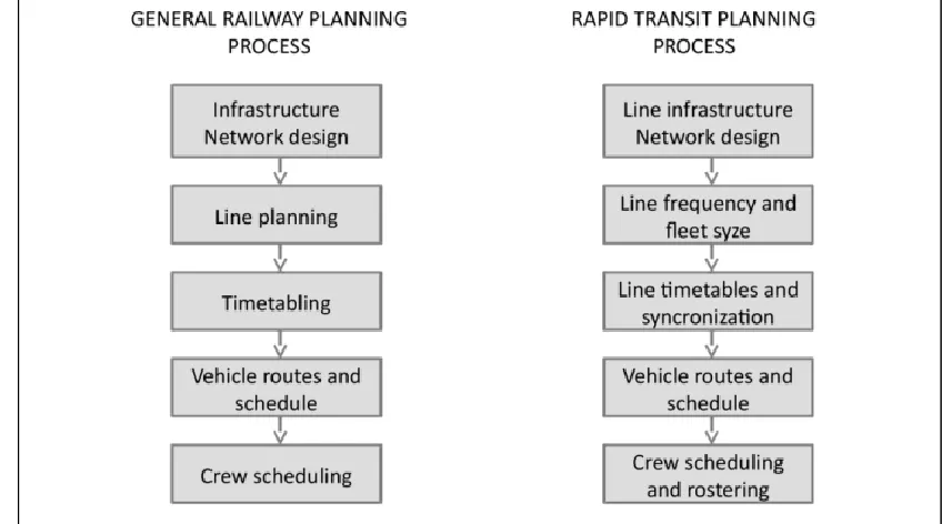
The planning process starts with the location of stations and tracks that join them. This is a pure network design problem that can be classified as an optimum network design for multi-commodity flow.
The second step is the line planning, which consists of choosing the origin, itinerary, stops, destination and frequency of each line. With this information, the exact time of arrival and departure from each station is fixed, thus constructing the timetable.
The following step is the design of train routes, in which a feasible sequence of line runs or services is obtained for a given period. Then the set of duties for the crew is determined. Finally, these duties are grouped into roster, which is a pattern of duties to be fulfilled for a certain number of consecutive days, Figure 1. Different goals give rise to different line planning problems. The two classical objectives
are to maximize the number of direct trips [1], and to minimize the cost [2]. However, the first one often leads to long travelling times, and the second is an only-operator oriented criterion. Minimizing travelling time is another classical objective, which has been considered in [3,4]. A review of the literature on line planning can be found in [5].
These lines may cross each other in some multiple stations usually at different levels, giving this way the possibility of a transfer from one line to the other. Thus, network design and line planning, except frequency setting, constitute the first step of the planning process, the second step being frequency and fleet size setting [6]. A second important difference between rapid transit systems and long and medium distance railways, is that in metropolitan areas several competing modes are available. Since metro passengers travel over short distance every day, one of their main concerns is travelling times, and their comparison with the travel times offered by other modes of transportation. This paper incorporates a mode choice based on a logit function. The objective is to decide the frequency and capacity of each line, maximizing the net profit of the system, which is computed as the difference between the revenue and the total cost. At first sight, this objective seems to be oriented to the operator. However, the profit itself is also a society oriented objective, because
Figure 1. General railway and rapid transit planning processes
International Journal of Railway Research (IJRARE) 3
it also maximizes the revenue, which in turns means maximizing the ridership. This way, a system maximizing the profit also attracts as many travelers as possible for whom the rapid transit system is better, in term of traveling time, than the alternative transportation modes. Therefore, the profit is also oriented to passengers.
The rest of the paper is structured as follows. In Section 2 the problem is formally described, and is modeled as a mathematical programming problem. Due to its extreme complexity, in Section 3 several algorithms are proposed to more efficiently solve the problem. These algorithms are tested and compared with each other in Section 4.
2. The Problem
2.1 Data and notation
In this section, the input data that are needed to define the Simultaneous Frequency and Capacity Problem (SFCP) are presented.
• Given is a set of connected lines L = {ℓ1, . . . ,
ℓ|L|} in the RTS. Let N = {i1, . . . , in} be the set
of stations that constitute the lines in L. In railway terminology, a line is characterized by two terminal stops, its itinerary and the train size. Other important aspects of each line ℓ are its length denoted by lenℓ and measured in length
units, and its number of stations associated, denoted by nℓ. Thus, the itinerary of each line ℓ
∈ L can be represented as {(i1, i2 ), (i2 , i3 ), . . . ,
(inℓ-1 , inℓ)}, where i1 , inℓ are the terminal stations
of the line, and {i1, i2, i3 , . . . , inℓ} and {inℓ, inℓ-1,
. . . , i1} define the two maximal paths of this line
in the network.
• Each couple of (directed) arcs (ij1, ij2) and (ij2,
ij1) define an (undirected) edge {ij1, ij2}. Let A be
the set of (directed) arcs, and let E = {{i, j}: i, j ∈ N, i < j, (i, j) or (j, i) ∈ A} be the set of edges defined from A.
• From these sets, an RTS is describes as the graph ((N, E), L).
• Let dij be the length of each arc (i, j) ∈ A. It is
assumed that dij = dji. The parameter dij can also
represent the time needed to traverse arc (i, j), transforming distances in times by means of the parameter λ, which represents the average
distance traveled by a train in an hour (commercial speed). The same value of λ for all trains is assumed. A parameter νℓ representing
the cycle time of line ℓ is considered and is, measured as the time needed for a train of line ℓ to go from the initial station to the final station and returning back. Thus, νℓ = 2 · lenℓ/λ.
• Let uci be the time spent in changing platforms
at station i.
• Let W = {w1. . . w|W |} ⊆ N × N be a set of
ordered origin-destination (OD) pairs, w = (ws,
wt). For each OD pair w ∈ W, gw is the expected
number of passengers per hour for an average day and is the travel time associated to w using the alternative mode, respectively.
• The passenger fare, the passenger subsidy (price that the government pays to the operator company for each trip) and the total number of hours that a train is operating per year are denoted by η, τ and ρ, respectively.
• The cost of operating one locomotive is cloc,
and the cost of operating one carriage is ccarr,
both per unit of length. The crew cost ccrew per
train and year is also given.
• The purchase cost of one locomotive is Iloc, and
one carriage is Icarr. A horizon of ρˆ years is
assumed for the purchase of trains to be recovered. A minimum number ymin of carriages for each train is considered.
• The capacity of a carriage is given by parameter Θ, measured in number of passengers seating and standing.
• A finite set of possible headways H for lines of the Rapid Transit System (RTS) is given.
2.2 The mathematical model
The problem can be modeled as a mathematical programming subject using the following sets of variables:
• xℓ∈ H is an integer variable representing the
headway of line ℓ (time between services, expressed in minutes).
4 International Journal of Railway Research (IJRARE) • yℓ∈ Z+ is the number of carriages used by each
train of line ℓ.
> 0 represents the travel time of pair w using the RTS network.
∈ [0, 1] is the proportion of OD pair w passengers using the RTS network, which depends on the travel time using the RTS (variable ) and on the travel time using the alternative mode (parameter uALT).
= 1 if the OD pair w traverses arc (i, j) ∈ A using line ℓ, 0 otherwise.
Note that these variables are set to zero whenever ( , )Ï ℓ, to reduce the size of the problem.
• = 1 if demand of pair w transfers at station k from line ℓ to line ℓ′, 0 otherwise. Note that these variables are set to zero whenever k does not belong to the two lines, nor when k is the origin or destination of pair w, in order to reduce the size of the problem.
The objective is the maximization of the net profit zNET defined as:
[ (h+t) ∑ ∈ − ∑∈ l ( + . ) − ∑∈ ( +
. ) − ∑∈ ] (1)
The first term in Equation (1) is the revenue zREV, which depends on the number of
passengers traveling (and therefore paying a ticket) in the RTS. The second term computes the rolling stock cost: the cost of operating the trains, which depends on the number of carriages. The last two terms are the fleet acquisition cost and the crew operating cost, respectively.
The constraints of the problem are:
≥ ∑:( , )∈ + ∑:( , )∈ − 1, ∈
, ≠ ∈ , ∈ ∩ , ≠ , (2)
:( , )∈ ∈
−
:( , )∈ ∈
=
0, ∈ \{ , } −1, = +1, =
(3)
≤ 60. .
∈
, ∈ , { , }
∈ (4)
= 1
1 + ( ), ∈ (5)
=
2
:{ , }∈ ∈
+ 60 l
{ , }∈ ∈
+
∈ ∩ :
∈ 2
+ , = ( , ) ∈ (6)
= [120. ⁄ l], ∈ (7)
≥ , ∈ (8)
> 0, ∈ ∈ , ∈
, ∈ {0,1}
∈ , { , } ∈ , ( , ) ∈ , ∈ , ∈ , ∈
Constraints (2) ensure that if an OD pair w enters station k ∈ N using one line, and exits from this station using another line, then a transfer is done. Equation (3) are the flow conservation constraints. Equation (4) imposes an upper bound on the maximum number of passengers that each line can transport per hour, which depends on the number of carriages and headway of this line. Constraints (5) represent the modal split, which uses the travel time described in Equation (6). Constraints (7) describe the required fleet for each line. A lower bound on the number of carriages for each line is forced by Constraints (8).
International Journal of Railway Research (IJRARE) 5
The maximization of Equation (1), subject to constraints (2)–(8), is a Mixed Integer Non-Linear Programming (MINLP) program that solves our problem. The nonlinearities of this model will be specified in Section 3.1, as well as some ways to avoid them.
3. Algorithms
In this section two different algorithms for solving the problem described in Section 2 are presented. The first one is based on efficient approaches of the mathematical model. It can be observed that the mathematical model described in Section 2.2 is operator’s oriented since each path associated to each OD pair is not necessarily the shortest path. On the other hand, the second algorithm takes into account the passenger point of view, by selecting the shortest path for each OD pair, yielding to solutions more realistic than the mathematical programming platform.
3.1 ILP-based algorithm
As mentioned, the MINLP presents several nonlinearities which can be avoided. In the following, such nonlinearities are described as well as the way for avoiding them.
1. In Constraints (4), the binary variable is multiplying the positive variable . This product can be easily linearized, by defining a new set of variables as follows:
≤ , ∈ , { , } ∈ , ∈ (9)
− 1 − ≤ , ∈ , { , } ∈ , ∈ (10)
≤ , ∈ , { , } ∈ , ∈ (11)
2. The definition of the proportion of passengers using the RTS, Constraints (5), uses the non-linear function logit. This nonnon-linearity is avoided by approximating the logit function by a linear function which takes into account three intervals on its abscissa axis as follows. Let z be the variable representing the travel time in the RTS and let F(z) = 1/(1 + exp(α - β( - z)) be the corresponding logit function for z. The piecewise linear function is defined as;
( ) ≔
1,
− 4 +
2 + 4 , 0,
(12)
∈
< −2
−2, +2
≥ +2
3. The required fleet described in Constraints (7), uses the ceiling function, which is non-linear as well, and the headway variables are in the denominator. This last nonlinearity can be avoided by fixing the headway of each line as a parameter.
Let ILP (x1 , ..., x|L|) be the model obtained
after avoiding the two first nonlinearities, in which the headway of each line ℓ, xℓ∈ H is fixed
as a parameter. The reader may note that the resulting program is an Integer Linear Programming model. Then, the algorithm presented in this section solves ILP (x1 , ..., x|L|),
for all feasible combinations of headways (x1 ,
..., x|L|) ∈ H|L|, keeping as a final output the best
solution found. The solution procedure is shown in Algorithm 1.
Data: As SFCF problem
For each combination of headways (x1 , ..., x|L|)
do solve ILP (x1 , ..., x|L|);
end
Result: arg ( ,..., | |) (x1 , . . . , x|L|)
Algorithm 1: Pseudocode for the ILP-based algorithm
3.2 A passenger’s oriented algorithm
At this stage, an algorithm is presented that solves the problem at hand by taking into account the passenger point of view. The idea is to iteratively check all possible combinations of headways as in the ILP (x1 , ..., x|L|) algorithm,
and once the headway is fixed, the demand is assigned in the RTS taking into account the shortest path associated to each OD pair. Later, the number of passengers traveling on each line and arc is computed. For each line, the arc with the highest number of passengers defines the minimum capacity that such line should have.
6 International Journal of Railway Research (IJRARE) Once these minimum required number of
carriages for each line has been calculated, the profit of the RTS can be easily computed. The Algorithm 2 shows its pseudo code.
Data: A railway system ((N, E), L), a set of possible headways H.
for each possible combination of headways do Let T = {} be the set for keeping solutions;
Compute the shortest path for each OD pair and the number of passengers traveling on each line and arc;
for each line ℓ do
Find the arc eℓ of ℓ with maximum load;
Find the minimum number of carriages needed to transport all passengers traversing eℓ;
end Compute the profit zNET ;
T = T ∪{zN ET};
end
Compute the maximum net profit;
Result: The combination of headways and capacities which yield the maximum profit.
Algorithm 2: Passenger’s oriented
4. Computational Experiments
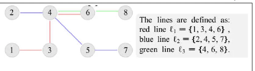
In this section a computational comparison between the two algorithms is presented, over ten small-size networks randomly generated. All these networks have been obtained from the topology described in Figure 2, which consists of eight stations and three lines. The number of passengers of each OD pair w was obtained
according to the product of two parameters: a parameter randomly chosen in the interval [5,15], by using a uniform distribution, whereas
the other one was randomly chosen in [51, 59], generating this way around 30.000 passengers for each instance. To define each arc length, the coordinates of each station were set randomly by means of a uniform distribution. So, the arc length at each instance is different since each arc connects to different positions of stations. The travel times using the alternative mode, were obtained by means of the Euclidean distance and a speed of 20 km/h, whereas, the travel time in the RTS were obtained according to the riding times with a speed of 30 km/h, the waiting time and the transfer time. Costs are based on the specific train model Civia as in [6].
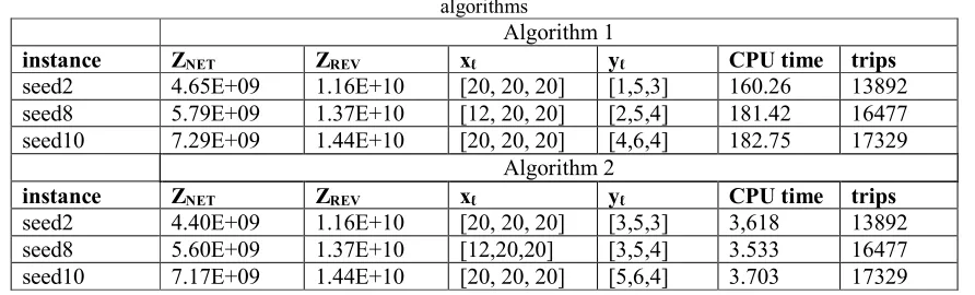
All the calculations for Algorithm 1 were performed in GAMS/CPLEX, whereas the Algorithm 2 was implemented in Java, both in a computer with 8 Gb of RAM memory and 2.8 Ghz CPU. In three of the ten instances, a difference in the solutions returned by both algorithms is observed. Note that, line ℓ1 and ℓ3
have a common track 4 - 6. In this track, travel times for Seed 2 and Seed 10 are the same over line ℓ1 and ℓ3, since both lines have the same
headway in the corresponding solutions. So, for trips traversing this track with the same travel time by ℓ1 and ℓ3, Algorithm 1 assigns
passengers on the most profitable line whereas Algorithm 2 assigns randomly passengers on line ℓ1 or ℓ3. In the Seed 8-instance, Algorithm 1
assigns passengers on a path that need not be the shortest path in the RTS, this algorithm might yield smaller number of carriages than Algorithm 2 and, therefore, better net profit.
5. Conclusions
It is reasonable to think that computational
experiments on medium-size networks could yield to solutions more interesting for analysis. So, as a future work, these algorithms will be tested over medium-size networks.
Figure 2. Line configuration used for the experiments
International Journal of Railway Research (IJRARE) 7 References
[1] M.R. Bussieck, P. Kreuzer, U.T. Zimmermann, Optimal lines for railway systems, European Journal of Operational Research 96, (1997), pp.54-63.
[2] M.T. Claessens, N.M. van Dijk, P.J. Zwanefeld, Cost optimal allocation of rail passenger lines, European Journal Operational Research 110, (1998), pp.474-489.
[3] J.-W Goosens, S. van Hoesel, L. Kroon, On solving multi-type railway line planning problems, European Journal of Operational Research 168, (2006), pp.403-424.
[4] A. Sch¨obel, S. Scholl, Line planning with minimal travel time. In 5th workshop on
algorithmic method and models for optimization of railways, number 06901, Dagstuhl Seminar proceedings, 2006.
[5] A. Sch¨obel, Line planning in public transportation, OR Spectrum 34, (2012), pp.491- 510.
[6] A. De-Los-Santos, G. Laporte, J.A. Mesa, F. Perea, Simultaneous frequency and capacity setting in uncapacitated metro lines in presence of a competing mode, Transportation Research Procedia, 3, (2014), pp.289–298.
Table 1: Summary of results for instances without the same solution for both algorithms
Algorithm 1
instance ZNET ZREV xℓ yℓ CPU time trips
seed2 4.65E+09 1.16E+10 [20, 20, 20] [1,5,3] 160.26 13892 seed8 5.79E+09 1.37E+10 [12, 20, 20] [2,5,4] 181.42 16477 seed10 7.29E+09 1.44E+10 [20, 20, 20] [4,6,4] 182.75 17329
Algorithm 2
instance ZNET ZREV xℓ yℓ CPU time trips
seed2 4.40E+09 1.16E+10 [20, 20, 20] [3,5,3] 3,618 13892 seed8 5.60E+09 1.37E+10 [12,20,20] [3,5,4] 3.533 16477 seed10 7.17E+09 1.44E+10 [20, 20, 20] [5,6,4] 3.703 17329