HISTOGRAM-BASED SMOKE SEGMENTATION IN FOREST FIRE DETECTION SYSTEM

HISTOGRAM-BASED SMOKE SEGMENTATION IN

FOREST FIRE DETECTION SYSTEM

Damir Krstini´c, Darko Stipaniˇcev, Toni Jakovˇcevi´c

and Naval Architecture University of Split

R. Boˇskovi´ca b.b., 21000 Split, Croatia

e-mail: [email protected], [email protected], [email protected]

Abstract.A focus of this paper is a pixel level analysis and segmentation of smoke colored pixels for the automated forest fire detection. Variations in the smoke color tones, environmental illumination, atmospheric conditions and low quality of the images of wide outdoor area make smoke detection a complex task. In order to find an efficient combination of a color space and pixel level smoke segmentation algorithm, several color space transformations are evaluated by measuring separability between smoke and non-smoke classes of pixels. However, exhaustive evaluation of the histogram-based smoke segmentation algorithms in different color spaces suggests that the peak performance is the distinctive feature of the algorithm itself rather than the algorithm-color space combination.

Keywords: smoke detection, image segmentation, histogram-based segmentation, colorspace evaluation, classifier design, Bayes classifier

I. INTRODUCTION

Forest fires represent a constant threat to ecological systems, infrastructure and human lives. According to the prognoses, forest fire, including fire clearing in tropical rain forests, will halve the world forest stand by the year 2030 [1]. Every year in Europe over 10.000 km2 _{of forest terrain is burnt} and in Russia and USA over 100.000 km2_{. The fact that} more than 20% of complete world CO2 emissions comes from forest fires indicates that it is a phenomenon which has to be dealt with great attention. The only effective way to minimize damage is early detection and appropriate fast reaction. Great efforts are therefore made in all regions to achieve early recognition. Different approaches and sensor inputs are used for the automatic detection of fire [2] [3], ranging from IR sensors to identify heat flux from the fire [4], light detection and ranging (LIDAR) systems [5] [6] that measure the laser light backscattered by the smoke particles, detection of smoke on satellite images [7], to smoke plume detection with cameras in visible spectra. Several platforms for surveillance activities have been tested in recent years. The individual method depends on the specific regional conditions and financial budget. Optical based systems often imply a high rate of false alarms due to atmospheric conditions (clouds, shadows, dust particle formations), light reflections and human activities. In systems based on visible spectra images, auto-matic smoke plume detection can be combined with human operator monitoring multi camera system. In addition, cost of the visual spectra camera equipment is often several times cheaper compared to IR cameras and other types of advanced sensors. Variation in the smoke color tones, environmental illumination, atmospheric conditions, quality of the images of wide outdoor areas and other problems make smoke detection a complex task. To detect smoke with reasonably low error rates, one has to implement several detection algorithms and a voting based strategy [1]. First processing step in smoke detection in most of forest fire detection systems is motion detection. Outputs of this processing are regions that are

detection candidates, which go through rest of processing and analysis procedures to determine if they have smoke characteristics. One of the commonly used techniques is the analysis of the obtained regions regarding color information in particular color-space. Smoke has certain visual characteristics relating to color and there are some rules which the color information of smoke adhere to. Such visual characteristics and rules are explored and analyzed in different color-spaces in order to better distinct between smoke and non-smoke regions. This process generally consists of two steps: (1) converting the image to the targeted color space and (2) classification of the image pixels according to the adopted model. The transformation of the image to a color space other than the RGB is assumed to increase separability between clusters of pixels representing different phenomena [8], thus improving the performance of image classification algorithm. The selection of the color space depends on the specific problem and algorithms used. A primary objective of this work is to evaluate performance of histogram based image classification algorithms for smoke detection task and to find color space-algorithm combination with lowest error rates. A framework for evaluation of different approaches in smoke detection is created and a dataset of images of forest fire is collected. The images are collected from various sources, taken in different conditions and with different equipment. All images in the dataset are segmented by hand in the ground truth segmentation and divided in the training and the testing set. The performance of the algorithms is measured using a receiver operating characteristics (ROC) [9] [10] [11] [12] [13] [14]. Acceptable error ranges are defined and algorithm performance examined at the error bounds. In order to select a particular color space with highest separability between smoke and non-smoke pixels, RGB color space is evaluated along with four other color space transformations: YCrCb, CIELab, HSI [8] and HS’I, which is a transformation of HSI. Based on the histogram analysis of the collected images, a transformation of the HSI color space is proposed in order to ISSN 1392 – 124X INFORMATION TECHNOLOGY AND CONTROL, 2009, Vol. 38, No. 3

HISTOGRAM-BASED SMOKE SEGMENTATION IN FOREST

FIRE DETECTION SYSTEM

Damir Krstini

ć

, Darko Stipani

č

ev, Toni Jakov

č

evi

ć

Faculty of Electrical Engineering, Mechanical Engineering and Naval Architecture,University of Split R. Boškovića b.b., 21000 Split, Croatia

e-mail: [email protected], [email protected]

Abstract. A focus of this paper is a pixel level analysis and segmentation of smoke colored pixels for the auto-mated forest fire detection. Variations in the smoke color tones, environmental illumination, atmospheric conditions and low quality of the images of wide outdoor area make smoke detection a complex task. In order to find an efficient combination of a color space and pixel level smoke segmentation algorithm, several color space transformations are evaluated by measuring separability between smoke and non-smoke classes of pixels. However, exhaustive evaluation of the histogram-based smoke segmentation algorithms in different color spaces suggests that the peak performance is the distinctive feature of the algorithm itself rather than the algorithm-color space combination.

Keywords: smoke detection, image segmentation, histogram-based segmentation, colorspace evaluation, classifier design, Bayes classifier.

1. Introduction

2

3

7

increase separability between smoke and non-smoke classes. The separability of smoke and non-smoke classes is measured using four statistical measures. The performance of two color histogram based image classification algorithms is evaluated. The first is the widely used lookup table method [10], and the second makes use of the Bayes decision theory [9] [10]. The performance of both approaches is evaluated in different color spaces, at four histogram resolutions. In order to improve the performance of the Bayes theory based classifier we adopt the kernel density estimation technique for calculating Bayes probability distributions. Suggested improvement aims to compensate the error introduced by the discretization of the color space.

II. ALGORITHMS USED FOR SMOKE DETECTION The performances of three histogram based algorithms are evaluated. For each algorithm a parametert is used to control algorithm sensitivity, where higher sensitivity implies lower rate of missed smoke-colored pixels, usually followed with higher rate of non-smoke pixels recognized as smoke. The exact meaning of the parameter t will be discussed for each algorithm separately.

The first algorithm is the simple Lookup Table Method (LT) [10]. This approach relies on the assumption that the smoke-colored pixels form an isolated cluster in some color space. The three dimensional histogram is created from the training set of the images using only pixels segmented as smoke in the ground truth segmentation (GT), defined manually by human operator. For each pixel marked as smoke in the GT segmentation, the appropriate cell in the histogram (discretized colorspace) is incremented. The lookup table is created by di-viding cell values with the largest value present. The values in theLTcells reflect the likelihood that the corresponding color range represents smoke. When classifying newly encountered images, pixel color triplet indexes the normalized value in the LT. A pixel is classified as smoke if this value is not less than a thresholdt. Thus, the parametertis defined as the minimum value whichLTcell indexed by a pixel color value triplet must have in order to be classified as smoke.

The second approach incorporates the probabilistic model for classification [9] to classify a pixel into the Smoke class (ωs) or into the Non-smoke class (ωns). Pixels belonging to the Smoke class are assumed to have measurement vector x

(color coordinates in some color space) distributed according to some distribution density function p(x|ωs, θs), where θsis the parameter governing the characteristics of the class ωs. Similarly, the distribution of the Non-smoke class is defined with p(x|ωns, θns), where θns defines the characteristics of the class ωns. Once the distributions have been estimated, the Bayes theorem [10] [15] is applied to calculate the probabilities:

p(ωs|x) =

p(x|ωs, θs)p(ωs)

p(x) (1)

p(ωns|x) = p(x|ωns, θns)p(ωns)

p(x) (2)

where the probabilities p(ωs) and p(ωns) are referred to as prior probabilities, since they represent the probabilities of

Smoke and Non-smoke classes before observing the vector

x. The naive Bayes (NB) classifier implicitly split the input spaceX into two decision regions with the decision boundary located along the contours where p(ωs|x) = p(ωns|x). The newly encountered pixel, represented with the measurement vectorx, is classified as smoke if

p(ωs|x)

p(ωns|x) >1 (3)

Prior probabilities p(ωs) and p(ωns) can be estimated from the training data: if a random sample of the entire population has been drawn, the maximum likelihood of p(ωs) is just the frequency with which ωs occurs in the training data set. In practice, real forest fires are very rare on any monitoring site, which would result inp(ωs)<< p(ωns). For the smoke detection task, the prior probabilities are used as a parameter to control sensitivity of the smoke detection algorithm. This way the algorithm can be biased to minimize more expensive errors (it is obviously more serious to misdetect a real forest fire than to disturb the operator with the false alarm). To be consistent with the LT method, the parameter t is set to t = p(ωns), where higher parameter values correspond to lower sensitivity of the detection algorithm.

Probability distributions for the Smoke and Non-smoke classes are computed from the training set of images, where smoke pixels are used to createSmokeclass distribution, while non-smoke pixels are used to createNon-smokeclass distribu-tion. Two separate color histograms are created representing Smoke and Non-smoke classes. Probabilities are computed directly from the histogram by dividing histogram cell values with the sum of all cells in the histogram. In the rest of the paper, this classifier will be referred to as NB1.

Alternative approach based on the assumption that the probability distribution at a continuity point can be estimated using the sample observation that falls within a region around that point utilizes the kernel density estimation technique [16], [17], [18]. Each input data sample (image pixel) is assigned a kernel, decreasing monotonically with the distance from the origin. Density at some pointxis computed as the sum of the contributions of all data samples:

fD(x) = 1

nhd n X i=1 K µ

x−xi

h

¶

, (4)

where n is the number of samples, his the bandwidth, and kernel K : Rd _{→ R, K(x) ≥ 0 is a symmetric function}

satisfying _Z

Rd

K(x)dx= 1 (5)

In the discrete histogram, pixel contribution is accounted for in a set of cells surrounding pixel origin in the targeted color space, rather than only in one cell. This approach is expected to compensate the error introduced by the discretization of the feature space, resulting in the probability distribution that better reflects the underlying true distribution. For the smoke detection task, each pixel, described by a three dimensional

2

3

8

2. Algorithms used for smoke detection

s

The performances of three histogram based algorithms are evaluated. For each algorithm, a parameter t is used to control algorithm's sensitivity, where higher sensitivity implies lower rate of missed smoke-colored pixels, usually followed with higher rate of non-smoke pixels recognized as smoke. The exact meaning of the parameter t will be discussed for each algorithm separately.

vector in some color space, is assigned a normal kernel

KN(x) = 1

p

(2π)3e −1

2kxhk2 (6)

Bandwidthhis connected with the histogram resolution

h= 1

N, (7)

whereN is the number of histogram bins in each dimension, and contribution of each pixel is calculated in 5 ×5 ×5 grid of cells centered on the cell corresponding to the pixel origin. Two histograms are created for SmokeandNon-smoke classes of pixels, and probability distributions are assessed by normalizing cell values of each histogram by dividing with the sum of all cells. It should be emphasized that additional computational costs are introduced only in the training phase of the classifier, while the classification process of newly encountered data remains the same. Classifier constructed using kernel density estimation technique will be referred as NB2 in the rest of the paper.

III. DATASET USED FOR TRAINING AND TESTING

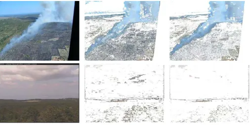
Fig. 1. Sample images with manually created Ground Truth (GT) segmen-tations. Smoke pixels are labeled white, non-smoke pixels are labeled black. Pixels labeled gray are not used in the experiments.

The total of 113 images in the dataset are divided into the training set, containing 64 images, and the testing set with 49 images. The complete dataset contains 87 images of real forest fires from the archive of the Professional Firefighting Brigade of the Split-Dalmatian county of the Republic of Croatia, and the rest of the images which do not contain fire have been taken on the potential locations of the forest fire surveillance system.

The ground truth (GT, see Fig. 1) is defined at pixel-level. The three labels method is adopted, where each pixel is labeled asSmoke(white),Non-smoke(black), orUndefined (gray). The Undefined label is assigned to pixels that are too ambiguous to be marked either way and to boundary pixels on the border between smoke and non-smoke regions. The image pixels labeled gray are not used in the experiments, either in the training phase, or in the testing phase. For images

containing no smoke, all of the image is labeled black ( Non-smoke).

IV. PERFORMANCE METRICS

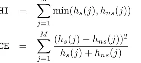
Two statistical measures are defined to evaluate overlap of the Smoke and the Non-smoke classes. In each color space two normalized histograms are created, representing mutually exclusive classes of pixels. The Histogram Intersection (HI) [19] [20] [21] and the Histogram χ2 _{Error (HCE) [19] [22]} are statistical measures of the overlapping of smoke and non-smoke histogram. Let M =N3 _{be the number of cells and}

h(j) value of cell indexed by index j. ThanHI andHCEare computed as follows:

HI = M X

j=1

min(hs(j), hns(j)) (8)

HCE = M X

j=1

(hs(j)−hns(j))2

hs(j) +hns(j)

(9)

For better separability of the classes, lowerHIand higherHCE

are desired.

The color histogram of the collected images is examined in several color spaces [8], including: RGB, HSI, YCrCb, and CIELab. Histogram analysis of the surveillance camera images of wide outdoor areas in the HSI color space shows that the low percentage of pixels corresponds to high saturated regions. Further, high saturated colors usually represent artificial ob-jects (like firefighting trucks) relatively close to the camera. Due to the atmospheric conditions, fog, particles in the air and other degradations of the image quality, distant regions and objects, which are of the main interest in the forest fire detection problem, are represented with low saturated colors. In order to increase separability between Smoke and Non-smoke classes, a transformation of the HSI color space is defined by (10):

S0₌ ½

2S, S <0.5

1, S ≥0.5 (10)

In the rest of the paper, this color space is referred to asHS0_I. The other two measures evaluate separability of classes with respect to the threshold value t, defined as in the lookup table algorithm. Absolute overlapping for some threshold t

is defined by

A(t) = B(t)

N , (11)

where B(t) is the number of histogram cells for which both smoke and non-smoke histogram have the value above thresholdt, andN is the number of histogram cells.

Relative overlapping is defined by

R(t) = B(t)

S(t), (12)

whereS(t)is a number of cells for which histogram represent-ing smoke has value above thresholdt. Relative overlapping is a ratio of the number of overlapping cells and the number of cells representing smoke, representing expected error rates. In calculating the absolute and the relative overlapping, histogram

2

3

9

3. Dataset used for training and testing

Figure 1. Sample images with manually created Ground Truth (GT) segmentations. Smoke pixels are labeled white,

non-smoke pixels are labeled black. Pixels labeled gray are not used in the experiments

4. Performance metrics

Two statistical measures are defined to evaluate overlap of the Smoke and the Non-smoke classes. In each color space two normalized histograms are created, representing mutual-ly exclusive classes of pixels. The Histogram Intersection (HI) [19] [20] [21] and the Histogram χ2

values are normalized to range [0,1] by dividing with the largest value present.

The performance of the algorithms is measured using a receiver operating characteristics (ROC). Each color space-classifier combination is evaluated at four histogram reso-lutions N = {32,64,128,256}. Smoke-Missed Error (SM) measures the number of smoke pixels that are not detected (False Negative).Non-Smoke Error (NS)measures the number of non-smoke pixels that are badly detected as smoke (False Positive). LetGTS be the number of pixels marked as smoke, andGTN S number of the pixels marked as non-smoke in the ground truth segmentation. LetM(t)be the number of missed smoke pixels, andE(t)number of non-smoke pixels detected as smoke at parameter value t. Than SM and NS errors are defined with

SM(t) = M(t)

GTS NS(t) =

E(t)

GTN S (13) ROC curve represents True positive vs. False positive char-acteristics for different values of the parameter t, where True positiveequals to1−SM(t)andFalse positiveequals toNS(t). Based on experiential results and testing, acceptable ranges for the SMandNSerrors are set to:

SM <0.2 N S <0.3 (14)

SM error bound is set to a lower value as it is more serious error to misdetect the smoke than to falsely detect non-smoke pixel as the non-smoke. However, the final decision about raising the alarm should be made by the post-processing decision system based on the output from the several smoke detection algorithms, where acceptable error ranges are defined separately for each algorithm.

V. COLORSPACE EVALUATION

Each color space is evaluated at four histogram resolutions in order to asses the ability of color space to separate smoke from non smoke pixels. HI andHCE results are presented in Table 1. The desirable result is lower HI value and higher

HCE value. The best result at each histogram resolution is highlighted in bold and underlined. The second best result is highlighted in bold.

In both measures, the results better than the results for

TABLE 1 COLOR SPACE EVALUATION

HI HCE

Res. 32 64 128 256 32 64 128 256

RGB .314 .261 .234 .226 1.120 1.251 1.325 1.348

YCrCb .351 .289 .252 .233 1.010 1.175 1.276 1.329 CIELab .380 .307 .265 .238 0.945 1.135 1.245 1.313 HSI .294 .257 .234 .227 1.164 1.269 1.326 1.346 HS’I .285 .251 .231 .226 1.187 1.284 1.335 1.347

the RGB color space are achieved in HSI color space and its derivatives, while other color space transformations achieve lower performance. According to both metrics, best performing color space is HS’I (Eq. 10).

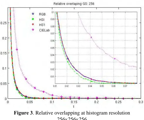
In Fig. 2 absolute overlapping is shown as a function of

thresholdt(Eq. 11) for histogram resolutionN = 256. Results are shown for RGB, HSI, HS’I and CIELab colorspaces. The relative overlapping (Eq. 12) for RGB, HSI, HS’I and CIELab color spaces at histogram resolution N = 256 is presented in Fig. 3.

At the highest histogram resolution the best results are

Fig. 2. Absolute overlapping at histogram resolution 256×256×256 (N= 256)

Fig. 3. Relative overlapping at histogram resolution256×256×256

achieved in the HSI color space, in both absolute and relative overlapping metrics. Overlapping is only slightly higher in RGB and HS’I color spaces. Similar results are achieved at other histogram discretization levels. At all histogram resolutions, the RGB color space achieves the result close to the best result for a particular resolution.

VI. ALGORITHM EVALUATION

Four sets of classifiers corresponding to different histogram discretization resolutions are generated. Each set containsLT classifier and two Bayes theory based classifiers (NB1,NB2) with different approaches in calculating density probability

240

5. Colorspace evaluation

Figure 2. Absolute overlapping at histogram resolution 256×256×256 (N =256)

Figure 3. Relative overlapping at histogram resolution 256×256×256

6. Algorithm evaluation

ROC curve represents True positive vs. False positive characteristics for different values of the parameter t, where

True positive equals 1−SM(t) and False positive equals NS(t). Based on experiential results and testing, acceptable ranges for the SM and NS errors are set to:

,

,

.

distribution. The classifiers are trained using 64 images in the training data set. The performance of the classifiers is evaluated using 49 images in the testing data set.

TABLE 2

AUCRESULTS, HISTOGRAM RESOLUTION32×32×32

Global AUC Local AUC

LT NB1 NB2 LT NB1 NB2

RGB 0.8333 0.8796 0.8582 0.0004 0.0886 0.0414 YCrCb 0.8273 0.8627 0.8406 0.0072 0.0586 0.0337 CIELab 0.8500 0.8569 0.8444 0.0192 0.0312 0.0385

HSI 0.8379 0.8818 0.8852 0.0137 0.1222 0.1093 HS’I 0.8385 0.8814 0.8838 0.0207 0.1139 0.1146

TABLE 3

AUCRESULTS, HISTOGRAM RESOLUTION64×64×64

Global AUC Local AUC

LT NB1 NB2 LT NB1 NB2

RGB 0.8376 0.8839 0.8860 0.0050 0.1179 0.1167 YCrCb 0.8400 0.8837 0.8683 0.0036 0.1190 0.0648 CIELab 0.8633 0.8836 0.8724 0.0294 0.1185 0.0775 HSI 0.8338 0.8865 0.8955 0.0047 0.1274 0.1705

HS’I 0.8330 0.8845 0.8934 0.0039 0.1255 0.1651

TABLE 4

AUCRESULTS, HISTOGRAM RESOLUTION128×128×128

Global AUC Local AUC

LT NB1 NB2 LT NB1 NB2

RGB 0.8301 0.8798 0.8952 0.0041 0.1264 0.1596

YCrCb 0.8356 0.8848 0.8921 0.0051 0.1352 0.1420

CIELab 0.8582 0.8850 0.8896 0.0408 0.1148 0.1452

HSI 0.8332 0.8798 0.8941 0.0056 0.1266 0.1584

HS’I 0.8340 0.8784 0.8921 0.0077 0.1242 0.1503

TABLE 5

AUCRESULTS, HISTOGRAM RESOLUTION256×256×256

Global AUC Local AUC

LT NB1 NB2 LT NB1 NB2

RGB 0.8300 0.8762 0.8920 0.0045 0.1216 0.1520

YCrCb 0.8284 0.8791 0.8942 0 0.1273 0.1600

CIELab 0.8507 0.8820 0.8964 0.0282 0.1323 0.1712

HSI 0.8256 0.8762 0.8897 0 0.1215 0.1440

HS’I 0.8298 0.8761 0.8875 0.0047 0.1218 0.1392

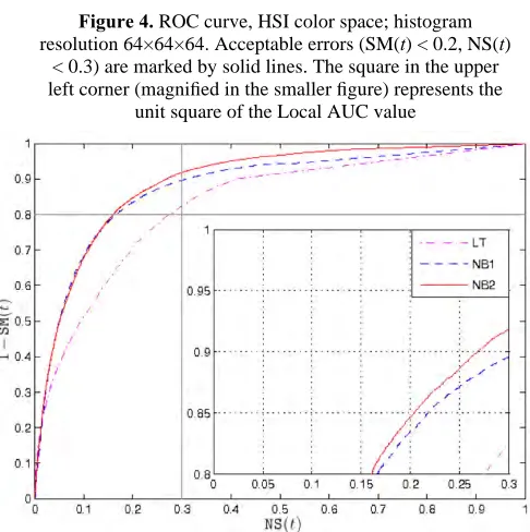
The classifiers are evaluated using a Receiver Operating Characteristics (ROC) curve analysis and Area Under Curve (AUC) value [11]. Global AUC is computed as the total area under the ROC curve within the unit square. The local AUC

[13] represents the area under the ROC curve within a square bounded by acceptable error ranges defined with equation (14), as shown in Fig. 4 and Fig. 5.

Error ranges are annotated by solid black lines, where top-left square of the graph corresponds to the acceptable error

Fig. 4. ROC curve, HSI color space; histogram resolution64×64×64. Acceptable errors (SM(t)<0.2,NS(t)<0.3) are marked by solid lines. The square in the upper left corner (magnified in the smaller figure) represents the unit square of the LocalAUCvalue.

Fig. 5. ROC curve, RGB color space; histogram resolution128×128×128. Acceptable errors (SM(t)<0.2,NS(t)<0.3) are marked by solid lines. The square in the upper left corner (magnified in the smaller figure) represents the unit square of the LocalAUCvalue.

ranges defined by (14). For each classifier, the global AUC is the total area under the ROC curve. The local AUC represents partition of the top-left square of the graph under the ROC curve. The results for the classifiers evaluated at different histogram resolutions are given in tables 2 trough 5. Each table contains the overview of the results of the classifiers at the particular discretization resolution. For each color space, the best result in global and local AUC metrics is emphasized in bold.

For color spaces with higher separability between the smoke and the non-smoke classes the improvement introduced by the kernel density estimation technique is observed at lower histogram resolutions, while theNB1performs better in color spaces with lower separability. At higher histogram resolutions theNB2 classifier outperforms theNB1classifier in all color spaces. In local AUC metrics, the peak performance of the

241

Figure 4. ROC curve, HSI color space; histogram resolution 64×64×64. Acceptable errors (SM(t) < 0.2, NS(t)

< 0.3) are marked by solid lines. The square in the upper left corner (magnified in the smaller figure) represents the

unit square of the Local AUC value

Figure 5. ROC curve, RGB color space; histogram resolution 128×128×128. Acceptable errors (SM(t) < 0.2,

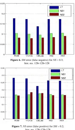
Fig. 6. SMerror (false negative) forN S= 0.3; hist. res.128×128×128

Fig. 7. N Serror (false positive) forSM= 0.2; hist. res128×128×128

NB2 classifier (Table 5; CIELab color space,N = 256) is up to 40% better compared to the peak performance of the NB1 (Table 4; YCrCb color space, N = 128).

Furthermore, these results suggest that no particular color space transformation can significantly improve classifying per-formance. For each color space, a particular resolution can be found where the classifier achieves its peak performance. For each classifier, the peak performances in all color spaces are close to each other, but they are achieved at different histogram resolutions. On the basis of this analysis, a conclusion can be made that the peak performance is the distinctive feature of the classifier itself, rather than the combination of the color space and the histogram resolution.

Smoke-missed (SM) error and non-smoke (NS) error on error boundaries defined by (14) are presented in Fig. 6 and Fig. 7.SM (False Negative)error forN S= 0.3 is presented in Fig. 6. The NB2 classifier achieves the lowest error rate in all color spaces. Fig. 7 shows N S (False Positive) error for SM fixed to0.2. The kernel density estimation technique improves performance in color spaces with higher separability. The lowest error rate is achieved by theNB2 classifier in the

RGB color space.

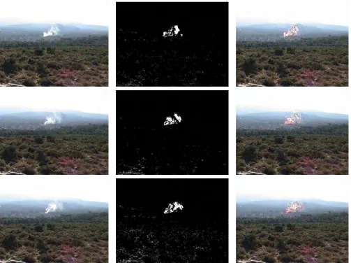
If the improvements inSMandN Serror rates are observed separately, it is obvious that benefits introduced by the NB2 classifier are higher with regard to N S error, i.e. less non smoke pixels are falsely detected as smoke. Examples of smoke segmentation using both versions of Bayes classifier are shown in Fig. 8.

The performance of the Bayes classifier with kernel density estimation technique is additionally evaluated by constructing a simple smoke detection algorithm. The algorithm is based on motion detection, where regions detected as ”moving” contain not only smoke but artefacts resulting from camera trembling, moving trees and bushes in the wind, sunlight reflections from particles in the air etc. After motion detection, detected regions are confirmed as smoke or rejected based on the output of the NB2classifier. Results are given in Fig. 9.

VII. CONCLUSION

The comparative evaluation of the histogram-based pixel level classification methods presented in this paper meets two goals. The first is the evaluation of different approaches in extracting knowledge from the training data set. Series of experiments confirm that the model for creating probability distributions using kernel density estimation technique im-proves the Bayes classifier performance. Classifying procedure of the Bayes classifier is not altered, and no additional com-putational costs are introduced in the decision-making phase. As expected, simple lookup table based classifier constructed solely from the smoke-labeled pixels achieves the lowest performance.

The second goal encountered is the selection of the algorithm-color space combination for the task of smoke detection. Thorough analyses suggest that peak performance is the distinctive feature of the classifier itself, rather than the classifier-color space combination. When selecting a color space for a particular task, balance should be found between memory requirements regarding histogram resolution and the efficiency of the required color space transformation. Good color space candidates for the smoke detection task are HSI and its derivative, as well as RGB color space.

The proposed algorithm is successfully implemented as one of the smoke detection methods of the Intelligent Forest Fire Monitoring System (iForestFire) [23] [24]. The algorithms described in this paper are only a part of the detection process and the final decision is made by result fusion of several different algorithms. Developed system is adopted as forest fire detection system for the coastline of the Republic of Croatia.

REFERENCES

[1] E. K ¨uhrt, J. Knollenberg, V. Mertens. An Automatic Early Warning System for Forest Fires. Annals of Burns and Fire Disasters, vol. XIV -n. 3,2001, 151-154.

[2] T. Celik, H. Demirel.Fire detection in video sequences using a generic color model. Fire Safety Journal, Vol. 44,2009, 147-158.

[3] B.-C. Ko, K.-H. Cheong, J.-Y. Nam. Fire detection based on vision sensor and support vector machines. Fire Safety Journal, Vol. 44,2009, 322-329.

[4] B. C. Arrue, A. Ollero, J. R. Martinez de Dios. An Intelligent System for False Alarm Reduction in Infrared Forest-Fire Detection. IEEE Intelligent Systems, Vol. 15, Issue 3,2000, 64-73.

2

4

2

Figure 6.SM error (false negative) for NS = 0.3; hist. res. 128×128×128

Figure 7.NS error (false positive) for SM = 0.2; hist. res. 128×128×128

7. Conclusion

Fig. 8. Sample result of smoke segmentation using pixel color classification. Columns left to right: input images; segmentations obtained usingNB1classifier; segmentations obtained usingNB2classifier. Classifiers thresholds are chosen at the ROC curve with True positive= 85%. Input image in second row contains no smoke

[5] A. B. Utkin, A. V. Lavrov, L. Costa, F. Sim˜oes, R. Vilar. Detection of small forest fires by lidar.Applied Physics B Lasers and Optics, Vol. 74, Issue 1,2002, 77-83.

[6] A. Lavrov, A. B. Utkin, R. Vilar, A. Fernandes.Evaluation of smoke dispersion from forest fire plumes using lidar experiments and modelling. International Journal of Thermal Sciences, Vol. 45,2006, 848-859. [7] K. Asakuma, H. Kuze, N. Takeuchi, T. Yahagi.Detection of biomass

burning smoke in satellite images using texture analysis. Atmospheric Environment, Vol. 36,2002, 1531-1542.

[8] A. K. Jain. Fundamentals of Digital Image Processing. Prentice-Hall, Englewood Cliffs, New Jersey,1989.

[9] D. J. Hand, H. Mannila, P. Smyth. Principles of Data Mining. The MIT press, Cambridge, Massachusetts,2001.

[10] S. Russel, P. Norvig. Artificial Intelligence, A Modern Approach. Pearson Education, Upper Saddle River, New Jersey,2003.

[11] J. Huang, C. X. Ling.Using AUC and Accuracy in Evaluating Learning Algorithms. IEEE Transactions on Knowledge and Data Engineering, Vol. 17, Issue 3,2005, 299-310.

[12] G. S. Rees, W. A. Wright, P. Greenway. ROC Method for the Evaluation of Multi-class Segmentation/Classification Algorithms with Infrared Imaginery. Electronic Proceedings of the 13th British Machine Vision Conference, University of Cardiff,2002, 537-546.

[13] C. E. Metz. Receiver operating characteristic analysis: a tool for the quantitative evaluation of observer performance and imaging systems. JACR - Journal of the American College of Radiology, Vol. 3,2006, 413-422.

[14] B. F. Buxton, W. B. Langdon, S. J. Barrett.Data Fusion by Intelligent Classifier Combination.Measurement and Control, Vol. 34, No. 8,2001, 229-234.

[15] S. Mitra, T. Acharya.Data Mining: Multimedia, Soft Computing, and Bioinformatics.John Wiley & Sons Inc., Hoboken, New Jersey,2003. [16] K. Fukunaga. Statistical Pattern Recognition. Handbook of Pattern

Recognition and Computer Vision, World Scientific Publishing Co., River Edge, New York,1993, 33-60.

[17] D. W. Scott, S. R. Sain.Multi-Dimensional Density Estimation. Hand-book of Statistics, Vol. 23: Data Mining and Computational Statistics, Elsevier,2004, 229-263.

[18] P. Meer. Robust techniques for computer vision. Emerging Topics in Computer Vision, Prentice Hall PTR,2004, 107-190.

[19] M. C. Shin, K. I. Chang, L. V. Tsap.Does Colorspace Transformation Make any Difference on Skin Detection. The 6th IEEE Workshop on Applications of Computer Vision,2002, 275-279.

[20] S. M. Lee, J. H. Xin, S. Westland. Evaluating of Image Similarity by Histogram Intersection. Color Research & Application, Vol. 30, No. 4, 2005, 265-274.

[21] M. J. Swain, D. H. Ballard.Color Indexing.Int. Journal of Computer Vision, Vol. 7, No. 1, 1991, 11-32.

[22] NIST/SEMATECH e-Handbook of Statistical Methods. http://www.itl.nist.gov/div898/handbook/,2006.

[23] D. Stipaniˇcev, T. Vuko, D. Krstini´c, M. ˇStula, Lj. Bodroˇzi´c. Forest Fire Protection by Advanced Video Detection System - Croatian Experi-ences. Third TIEMS Workshop - Improvement of Disaster Management System, Trogir,2006, 26-27.

[24] Lj. Bodroˇzi´c, D. Stipaniˇcev, D. Krstini´c. Data fusion in observer networks. MASS07, The 4th IEEE International Conference on Mobile Ad-hoc and Sensor Systems, Pisa, Italy,2007, 8-11.

2

4

3

Figure 8. Sample result of smoke segmentation using pixel color classification. Columns left to right: input images; segmentations obtained using NB1 classifier; segmentations obtained using NB2 classifier. Classifiers thresholds are chosen

2

4

4

Figure 9. Smoke detection based on the motion detection and the Bayes classifier with the kernel density estimation technique. Columns from left to right: input images; motion detection; smoke regions confirmed with NB2 classifier implemented in

HSI colorspace, hist. res N = 64

Received February 2009.