Volume 01, No.7, July, 2015
P
age
18
Variance Function of the Difference between Two estimated
responses in regulating Blood Sugar Level in a Diabetic patient
using Herbal Medicine
A. Karanjah*, F. Njui** and G.P. Pokhariyal***
University of Nairobi. Kenya
ABSTRACT
In this paper response surface methodology was employed to investigate effectiveness of herbal medicine (Aqueous extract of Ganotech- from medicinal mushroom) in reducing the blood sugar level of a diabetic to acceptable level. In this setup, observations are made to investigate effectiveness for particular dosage at reducing the blood sugar level with time. The variance function comes in handy as a tool for discrimination between two points on the identified response surface. The most feasible of all the identified point of equal yield is the one in which the variance function is minimal. In this study we use the variance function of the difference two points to provide reliable advice on the range around which the dosage is desirable and time required to effectively reduce the blood sugar level to acceptable range. The analysis of the data from the experiment indicates that 46.2492 mg/dl concentration of the herbal medicine is effective in regulating blood sugar level in a diabetic within 136.1304 minutes to acceptable range.
Key words: Response surface; Variance function; Diabetes; Herbal-Medicine; Treatment.
2000 Mathematics Subject Classification: 62K15, 62K20
1. INTRODUCTION
Medicinal herbs constitute an important source of raw materials for both the traditional and the conventional medicine. They have been in use world over, however over reliance on herbal drugs whose active ingredients have not been quantified results to different herbalist prescribing different concoctions depending on the flora availability. This may lead to resistance development, overdose or under dose which may lead to negative repercussion. There is need to standardize commonly used herbal drugs, by formulating a mathematical model that can be used to determine the best combination of herbs and best preparation practices in order to achieve the optimal response. By so doing, useful results and conclusions can be drawn by planned and designed experiment.
Volume 01, No.7, July, 2015
P
age
19
measured response variables and several explanatory factors to obtain an optimal response by using a series of tests. The main advantage is to reduce the required experimental runs and to optimize formulation design in pharmaceutics studies.
An experiment based on a herbal medicine extracted from Medicinal Mushrooms referred to as Aqueous extract of Ganotech, was carried out involving 21 albino rats. The rats were grouped into four groups all induced with diabetes as per standards and procedures required in a laboratory. After the recording of the Fasting Blood glucose the treatments were carried on the animals as per grouping and dosage levels effected using the herbal extract with varied concentrations of 25 mg/Kg, 50 mg/Kg and 75 mg/Kg. The fourth group (control group) was treated with conventional drug Metformin 500mg/Kg. The readings of the Oral Glucose
Tolerance Test (OGTT) were undertaken at and minutes, which
availed the data in use.
2. THE MODEL
In any treatment arrangement, we seek a treatment or treatment combination that can be used to either reverse a condition, eradicate or arrest a condition in order to minimize suffering or to help the patient bear a condition with less pain. The aim is to regulate the blood sugar level of a patient at that particular time to a level that is acceptable according to medical standards. Observations are made so as to note how effective the particular amount/concentration of the identified herbal drug is at reducing the blood sugar level with time. This investigation therefore is used to determine;
i). The best possible level of concentration of the identified herbal medicine and
ii). Time taken, to regulate the blood sugar level to within acceptable level in a diabetic.
The results will provide the most reliable advice ( on the basis of the findings) on the range around which the dosage is desirable so as to make use of the information in maintenance of the desired level of glucose in a diabetic patient.
In most Response Surface Methods (RSM) problems, the true response function is
unknown, we therefore need to approximate the function. In order to develop a proper approximation for , we model the data by starting with a low-order polynomial in some small region. If the response can be defined by a linear function of independent variables, then the approximating function is a first-order model. With reference to any order polynomial regression model (design) the general design for given observations is given as
Volume 01, No.7, July, 2015
P
age
20
The parameter measures the expected change in response per unit increase in when the
other independent variables are held constant. The -th observation and -th level of
independent variable is denoted by .
However, if a first order model is not sufficient and curvature exists, then a higher order model needs to be fitted to the data to explore the nature of the response surface. The data used suggested curvature and hence a higher order model is explored. One such model is the second order model which is of the form;
Specifically with two predictor variables, equation (4) is of the form,
where is the parameter associated with the interaction effect between concentration and
time.
3. PARAMETER ESTIMATES
The method of least squares is practically employed to estimate the regression coefficients in (5). However, using statistical software, Design of Experiment (DoE) for the regression analysis, the same results will be easily obtained.
Volume 01, No.7, July, 2015
P
age
21
Table 1.1 Parameter Estimates for the Quadratic model
Factor Estimate d.f S. Error 95 % LCL 95 % UCL
Intercept 0.3371 1 0.052 0.23 0.44
Time 0.1591 1 0.027 0.10 0.21
Concentration 0.0535 1 0.026 0.001389 0.11
0.0687 1 0.031 0.003348 0.13
0.1102 1 0.044 0.021 0.20
-0.00144 1 0.050 -0.100 0.100
The regression equation generated is
where the variables as time represented by A and the as concentration respectively. The
corresponding analysis of variance table generated from this data is as follows:
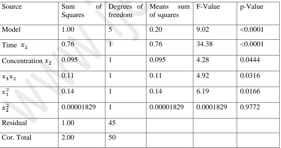
Table 1.2 ANOVA for Response Surface Quadratic model
Source Sum of
Squares
Degrees of freedom
Means sum
of squares
F-Value p-Value
Model 1.00 5 0.20 9.02 <0.0001
Time 0.76 1 0.76 34.38 <0.0001
Concentration 0.095 1 0.095 4.28 0.0444
0.11 1 0.11 4.92 0.0316
0.14 1 0.14 6.19 0.0166
0.00001829 1 0.00001829 0.0001829 0.9772
Residual 1.00 45
Volume 01, No.7, July, 2015
P
age
22
4.1 Tests of hypotheses-Model Adequacy
Using these results of Table 1.2 for the second order model obtained in (5), the test of hypothesis can be carried out for this model as well as the parameter estimates. The hypothesis for the model is stated as:
, against for at least one .
The calculated value of the test statistic . We thus reject the
null hypothesis. Therefore model is significant. Alternatively using the generated -value we confidently state that the Model F-value of 9.02 implies the model is significant and there is only a 0.01% chance that an F-value which is this large could occur due to error (noise).
The coefficient of determination is , indicates that 50.06 % of the variation in
the sugar level is accounted for by the model (or is due to the variation in time and
concentration).
4.2 Test of hypothesis on individual parameter estimates
We compute the test statistic for each parameter estimate and compare the resulting values with the table values at the desired level of significance ( ) and accompanying degrees of freedom from the model used. However, this can equivalently be achieved by using the confidence interval in which we find that provided that the confidence interval does not include zero then the parameter estimate is significant otherwise it is not. The test hypothesis for individual parameter estimates is stated as
, against
Using the confidence interval approach we find that the parameter estimates that are
significant are the ones corresponding to the variables and That is to imply
that the variables which contribute to the reduction of blood sugar level are time, concentration, time squared and interaction of concentration with time. The parameter estimate corresponding to concentration squared is not significant, which implies that the accompanying variables do not explain the variation of blood sugar level individually.
5. ANALYSIS OF THE STATIONARY POINT OF THE SECOND-ORDER MODEL
When there is a curvature in the response surface the first-order model is not sufficient. Thus, a second-order model becomes useful in approximating a portion of the true response surface with parabolic curvature. Using statistical software (Design of Experiments-DoE) in analysis of a quadratic response, we get the following three dimension plots for the two continuous
Volume 01, No.7, July, 2015
P
age
23
Figure 1. Three d-surface plot View
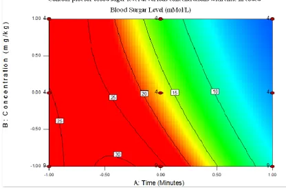
The accompanying contour plot for the three dimension view is as follows:
Volume 01, No.7, July, 2015
P
age
24
The three dimension plot suggest that curvature exists and hence justification for having fitted the second order model. The second-order model is flexible, as it takes a variety of functional forms and approximates the response surface locally which is a good estimation of the true response surface.
From the above results we conclude that response surface is explained by the second-order model. We now determine the optimum setting and recommend it for the effective management of average sugar level in a diabetic patient. Graphical visualization of contour plots helps in understanding the second-order response surface. Specifically, three dimensional surface plot and their accompanying contour plots help characterize the shape of the surface, and through these we will be able to approximately locate the optimum response. Using the fit of the second-order models, we illustrate quadratic response surfaces such as minimum, maximum, ridge, and saddle point. In the case that an optimum exits, then this point is a stationary point which can result in any of the aforementioned four possibilities. The stationary point in response surface models is the combination of design variables, where the surface is at either a maximum or a minimum in all directions. If the stationary point is a maximum in some direction and minimum in another direction, then the stationary point is a saddle point. When the surface is curved in one direction but is fairly constant in another direction, then this type of surface is called ridge system (Oehlert 2000).
The stationary point is evaluated by use of matrix algebra for which the fitted second order model (5) in matrix form is expressed as follows:
The derivative of with respect to the elements of the vector is given by
Therefore, the solution to stationary point is
where is a vector of the first-order regression coefficients and is a
symmetric matrix whose main diagonal elements are the quadratic coefficients and
whose off diagonal elements are one-half the mixed quadratic coefficients ,
Montgomery (2005). As a result, the estimated response value for the fitted model at the identified stationary point is obtained as:
Volume 01, No.7, July, 2015
P
age
25
One of the points of interest in this study is the minimum condition for the explanatory
variables. The results used above are for a maximum condition, modifying equation for a
minimum condition by negating it so as to achieve our desired results, the stationary point solution with this modification is found to be as follows:
We now find the stationary point in terms of the natural variables, time and concentration
from the coding concept adopted earlier. For time as a variable, we have
This implies that the time taken to reduce the blood sugar level to within acceptable range is
136.1304 minutes. With respect to concentration we have,
Thus 46.2492 mg/dl of the herbal formula is to be used to regulate the blood sugar level to within the acceptable range.
As a result, the estimated response value at the stationary point is given as
Volume 01, No.7, July, 2015
P
age
26
where is the mean response given in equation (15), is as in equation (12) and is
provided in equation (11). The reversed transformation for the amount of blood sugar level coded gives us
)
This is the estimated minimum blood sugar level for the given predictor variables.
6.1 Variance of Estimated Response
The variance function of the fitted model in a general case is used to evaluate competing designs, whereby the best design is one which has the smallest possible variance. The
variance of estimated response at a point on the sphere of radius ρ where,
is
here is assumed to be unknown but constant and are taken to be
non-stochastic. The prediction variance of the estimated response at a point say is given by,
where is the vector of co-ordinates of a point in the design space expanded to model form. Mostly, experimenters opt to use scaled predicted variance (SPV) arrived at by multiplying
(18) by the design size and then dividing through by the process variance , that is
This scaling is widely used to facilitate comparisons among designs of various sizes and
eliminates the need to know the value of .
Using the observations vector for the stationary point given in equation (12)
The corresponding observation vector generally constructed from for the quadratic model
Volume 01, No.7, July, 2015
P
age
27
From (20), the variance is computed using
Thus,
We now show that is minimum by comparing it with variance of another point on the
same response surface. We take point which is different from the stationary point, but in
the neighbourhood of this stationary point, where,
Volume 01, No.7, July, 2015
P
age
28
Comparing the results of equation (22) and (24), it clearly shows that the variance of the estimated response arising from the vector in equation (21) that is generated from the estimated response in (12) is a minimum as compared to that generated by the vector of (23) on the same response surface. Thus is minimum.
6.2 Variances Function of the Difference between two Estimated Responses
Suppose that and are two row vectors of the form of a row of but which arise
from two distinct points identified on two estimated response surfaces of different radii. Then
Similarly
Let
denote the variance of the difference between the two estimated responses (25) and (26) at the points and . This variance simplifies to
When the design is rotatable, then has a special form (Box and Hunter (1957) and the
variance as stated in equation (28) is invariant under orthogonal rotations in the predictor space, Herzberg (1967).
Taking the expression of (25) and that of (26) to be the points described in and
of (21) and (23) respectively, then the variance in (28) for this specific test run is
computed for as follows;
Volume 01, No.7, July, 2015
P
age
29
7. CONCLUSION
It was found that equation (30) yields the variance function of the difference between two estimated responses and the difference of the variance functions between two estimated responses for the herbal drug extract from medicinal mushrooms. However, by selecting the one that provides a minimum we emphasize that the variance function of the difference between two estimated responses should be used in selecting an optimal model in the effective management of diabetes using herbal drug extract from medicinal mushrooms. The selection of any vector other than that of the stationary point will provide the region within which the factors of interest can be varied provided that the variance is minimize. Hence, this would act as a suitable guide to determine the range within which factors of interest should be varied.
If we consider points close together in the factor space, an optimal design with regard to rotatable design in two dimensions from this approach will be chosen on the basis of minimum variance function criterion as emphasized by Herzberg (1967), Box and Draper (1980), and, Huda and Mukerjee (1984).
Research funded by the National Commission for Science, Technology and Innovation.
8. REFERENCES
i. Box, G. E. P. and Draper N. R. , The variance function of the difference between two
estimated responses. Journal of the Royal Statistical Society, B 42 (1980), 79-82
ii. Box, G. E. P. and Hunter, J. (1957). Multi-factor experimental designs for exploring
response surface. Annals of Mathematical Statistics. 28 , 195-241,.
iii. Herzberg A. M. (1967), The behaviour of the variance function of the difference
between two estimated responses. Journal of the Royal Statistical Society, B 29 , 174-179.
iv. Huda S and Mukerjee R, Minimizing the maximum variance of the difference
between two estimated responses, Biometrika, 71,(1984), 381-385.
v. Montgomery Douglas, C. (2005). Design and Analysis of Experiments response
surface methods and design. John Willey and Sons Inc. New Jersey.
vi. Karanjah, A. , Njui, F. and Pokhariyal, G. P. (2008). The variance function of the
difference between two estimated responses for a fourth order rotatable design in two dimensions. Far East Journal of Theoretical Statistics, Vol. 26, Iss. 2, Pages 177 – 191.
vii. Oehlert, Gary W. (2000). Design and analysis of experiments: Response surface
design. New York. W.H. Freeman and Company,
viii. Saeed Ghanbarzadeh, Hadi Valizadeh and Parvin Zakeri-Milani. (2013). Application of