Non-parametric context-based object classification in images

(1)

Information Technology and Control 2017/1/46 86

Non-Parametric

Context-Based Object

Classification in Images

ITC 1/46

Journal of Information Technology and Control

Vol. 46 / No. 1 / 2017 pp. 86-99

DOI 10.5755/j01.itc.46.1.13610 © Kaunas University of Technology

Non-Parametric Context-Based Object Classification in Images

Received 2016/09/11 Accepted after revision 2017/02/20

http://dx.doi.org/10.5755/j01.itc.46.1.13610

Toma Rončević

University of Split, University Department of Professional Studies, Livanjska 5, 21000 Split, Croatia tel.: +385914433840, e-mail: [email protected]

Maja Braović

University of Split, Faculty of Electrical Engineering, Mechanical Engineering and Naval Architecture Ruera Boškovića 32, 21000 Split, Croatia

Darko Stipaničev

University of Split, Faculty of Electrical Engineering, Mechanical Engineering and Naval Architecture Ruera Boškovića 32, 21000 Split, Croatia

Corresponding author: [email protected]

Segmentation and classification of objects in images is one of the most important and yet one of the most com-plex problems in computer vision. In this work we propose a new model for natural image object classification using contextual information at the level of image segments. Context modeling is largely independent of ap-pearance-based classification and proposed model enables simple upgrade of existing systems with informa-tion from global and/or local context. Context modeling is based on non-parametric use of appearance-based classification results which is a novel approach compared to previous systems that model context on a limited number of rules expressed with a fixed set of parameters. Model implementation resulted in a system that, in our simulations, showed stable improvement of the appearance-based object classification.

(2)

87 Information Technology and Control 2017/1/46

Introduction

Object classification in natural images is generally a very complex problem due to variations in object ap-pearance when viewed from various perspectives, changes in scene illumination and typically a large number of partially occluded objects in a scene. Com-mon approaches to object classification rely heavily on the visual characteristics that can be associated with the objects that need to be classified, but the object appearance alone is usually not enough to recognize it reliably and unambiguously. To aid this, contextual in-formation can be used in order to improve recognition. Papadopoulos et al. in [19] explained image context as:

“Image context includes all possible information sources that can contribute to the understanding of the image content, complementarily to the use of the visual features.”

Studies of human vision showed that context is used on different levels of image understanding and that it is possible to distinguish between several kinds of contextual interactions: semantical (related objects usually appear together in the same image, for exam-ple keyboard and a computer mouse), spatial (key-board is usually in front of the computer screen) and orientational (chair in front of the computer is usu-ally facing the computer screen) (subset of relations presented in [4]). From the perspective of computer vision it is possible to connect different types of tasks such as image classification, image segmentation, de-tection, localization and recognition of objects with the use of different types of context. There are mul-tiple ways in which one could divide different types of context. One can differentiate between local and global context or between levels of context in relation to the levels in the hierarchy of the image (e.g. scene [3], objects [13], regions [27], object features [28] and pixels [21]). It is also possible to differentiate between sources of contextual information or the nature of ob-jects in a scene [29]. Generally, in analogy with human vision, contextual information can improve the speed and robustness of algorithms that are based on the analysis of object appearance. That is most evident in cases where the object appearance is compromised with low image quality or the complexity of the scene (occlusions, shadows, bad lighting) where human vi-sion copes much better [4]. A taxonomy of sources of contextual information used in image processing and understanding is given in [6], while a critical survey of

context-based natural image parsing is given in [20]. The proposed model introduces several novelties compared to the previous models used for con-text-based object classification. The first novelty is the use of non-parametric methods for the inclusion of local contextual information with the necessary appearance-based object classification. Non-para-metric approach is already partially explored in [24], but the described model of the basic classifier (k-Nearest Neighbors) did not give good results on a smaller image dataset (Stanford Background Data-set) and it used Markov random field for the inclusion of local context. The second novelty is the use of the results of feature-based segment classification as di-rect features that represent the local context followed by use of unsupervised learning (k-modes algorithm [14]) for approximation of the class probability. To our knowledge, this approach has not been used in any other previous work.

The following sections are structured as follows: in the second section we present our non-parametric context-based model for object classification, and give information about image segmentation methods, image features, local context and global context that we used in its implementation. In the third section we validate the presented model, and in the fifth and final section we give conclusions and discuss future work.

Proposed model

(3)

nodes and connected by directed edges that describe the conditional dependency between the two vari-ables. The NACC model is constructed to classify a relatively small part of the image that represents the object or a part of the object in the image, and belongs to one of the predefined classes. Dependences be-tween random variables are based on the following observations:

_ Edge C → X represents the conditional probability P(X|C) that shows our expectations about the appearance of the object in the image, given the object class.

_ Edge L → C represents the conditional probability P(C|L) that shows our expectations about the object class, given the local context of the object.

_ Edge G → L represents the conditional probability P(L|G) that shows our expectations about the local context of the object, given the global context of the image.

_ Edge G → C represents the conditional probability P(C|G) that shows our expectations about the class of the object, given the global context of the image.

_ Edge G → X represents the conditional probability P(X|G) that shows our expectations about the appearance of the object, given the global context of the image. This dependency describes how illumination, distance or type of the scene can affect the features related to the object appearance. For example, the way that the sky looks depends on the time of the day, weather conditions or the sun position in relation to the camera.

Figure 1

NACC model represented as a probabilistic graphical model

ܿ௠௔௫ൌ ݉ܽݔ஼ܲሺܥ ൌ ܿȁܩǡ ܮǡ ܺሻ (1)

ܲሺܥǡ ܩǡ ܮǡ ܺሻ ൌ ܲሺܩሻܲሺܮȁܩሻܲሺܥȁܩǡ ܮሻܲሺܺȁܩǡ ܥሻ (2)

ܲሺܥȁܩǡ ܮǡ ܺሻ ൌ௉ሺீሻ௉ሺ௅ȁீሻ௉ሺ஼ȁீǡ௅ሻ௉ሺ௑ȁீǡ஼ሻ_{௉ሺீǡ௅ǡ௑ሻ} (3)

ܲሺܥȁܩǡ ܮǡ ܺሻ ൌ ߙԢ௉ሺ஼ȁீǡ௅ሻ௉ሺ஼ȁீǡ௑ሻ_{௉ሺ஼ȁீሻ} (4)

ߙԢ ൌ௉ሺ௅ȁீሻ௉ሺ௑ǡீሻ_{௉ሺீǡ௅ǡ௑ሻ} (5)

Figure 2. Overview of the NACC model

Equation (1) is the base of the classification of image objects (or parts of the image objects). The object is classified according to the maximum probability of class given the object’s global context, local context and appearance. The equations (2)-(4) represent the product of all conditional probabilities that result from the Bayesian network, and they show how the final probability for the class of the object is acquired. Equation (5) represents the normalizing factor that does not depend upon the class of the object, and since it is the same for all classes we omit it from fur-ther calculations.

ܿ௠௔௫ ൌ ݉ܽݔ஼ܲሺܥ ൌ ܿȁܩǡ ܮǡ ܺሻ (1)

Figure 2. Overview of the NACC model

(1)

(2)

(3)

Figure 2. Overview of the NACC model

(4)

(5)

A general overview of the NACC model is shown in Figure 2.

Figure 2

(4)

Conditional probabilities P(C|G, L), P(C|G, X) and

P(C|G) should be modeled in order for a NACC model to be implemented. These probabilities can be learned by machine learning methods on a set of images. In practice, however, it is often the case that we cannot approximate these probabilities with the desired accuracy on the account that we do not have enough data (i.e. labelled images) on which to learn these probabilities. Therefore, a model that is simpler should be considered, and a simpler model was indeed used while testing our system on a set of training images. Our simpler model did not take into the account the global context of the image, but rather assumed that the global context is the same for all of the images and few global features were in-cluded in appearance base classification (absolute position of segment). The reason for this simplifica-tion is that it is not simple to describe and to deter-mine the types and the number of types of the global context, and neither is it simple to distinguish and reliably classify an image into one of these types on the basis of some of the image features. To fit this simpler model, we transformed the equations (3)-(5) into the equations (6)-(8):

ܲሺܥȁܮǡ ܺሻ ൌ௉ሺ௅ሻ௉ሺ஼ȁ௅ሻ௉ሺ௑ȁ஼ሻ_{௉ሺ௅ǡ௑ሻ} (6)

ܲሺܥȁܮǡ ܺሻ ൌ ߙԢ௉ሺ஼ȁ௅ሻ௉ሺ஼ȁ௑ሻ_௉ሺ஼ሻ (7)

ߙԢ ൌ௉ሺ௅ሻ௉ሺ௑ሻ_{௉ሺ௅ǡ௑ሻ} (8)

ܲሺܥ ൌ ܿሻ ൌ௔_௕ (9)

݈݋݃ܲሺܥȁܮǡ ܺሻ ൌ ߙܽଵ൅ ߚܽଶെ ܽଷ. (10)

(6)

݈݋݃ܲሺܥȁܮǡ ܺሻ ൌ ߙܽଵ൅ ߚܽଶെ ܽଷ. (10) (7)

where P(C) represents the frequency with which the class appears in the training set, and is calculated for each of the classes as shown in equation (9):

where a is the number of pixels or segments that be-long to class c, while b is the total number of pixels or segments.

Since the equation (7) is based on the approximations of the distributions P(C|L), P(C|X) and P(C), it would be useful to add to the model certain parameters that

can be used to regulate representations of certain dis-tributions in the final distribution P(C|L, X). Since we are only interested in a class that maximizes equation (7), monotony of the logarithmic function can be used and the equation can be represented in the form of equation (10):

In the equation (10), a1= P(C|L), a2= P(C|X), a3= P(C), and α and β are parameters that can alleviate or em-phasize the approximated distributions in regards to the distribution P(C) whose weight parameter is normalized to 1. This equation sums up the model im-plemented in this work. α and β parameters were de-termined during model validation by cross-validation and our results were obtained for α =30 and β =0.4. Image segmentation

Image segmentation is one of the essential steps in image processing. It is a process that divides the im-age into smaller parts according to some given logic. For example, the image can be divided into segments of uniform color and/or texture, or into segments that represent objects in the image. In practice, it is often preferred to first segment the image into segments of approximately equal sizes, where each segment would have approximately equal pixel features, and then combine these segments into objects.

In the proposed model, image segmentation methods we used were uniform grid segmentation and super-pixel-based segmentation.

(5)

our uniform segments was around 10x8 pixels. We also experimented with different sizes of the seg-ments (16x16 and 64x64), but we did not notice a sig-nificant change in the classification results.

Superpixel-based segmentation divides the image into segments of irregular shape, size and position in the image, but on the other hand these segments encapsulate pixels with similar image features (e.g. color or texture), and can contain partial information about the shape of the object. By unifying superpix-els one can get the precise segmentation of the entire object. A method that we used for superpixel-based segmentation is Simple Linear Iterative Clustering (SLIC) [1], but in our proposed model this algorithm is completely independent of the rest of the model and implementation and it can easily be replaced by another algorithm that can perform accurate object segmentation.

In the proposed model, the entire learning process and appearance-based and local context-based clas-sification is conducted on segments obtained by uniform grid segmentation of the image. Superpix-el-based segmentation is used in the later stage where it is superimposed on the uniform grid segmentation. Every superpixel is assigned with a class label by us-ing a method of majority votus-ing by pixels inside the superpixel or by using naive Bayes classifier at the pixel level, as shown in equation (11), where PSP(C) is the probability of the class of the superpixel SP, and

Pi(C) is the probability of the class of the pixel i that

belongs to the superpixel SP:

�� ∏�� . (11) (11)

Appearance-based object classification For appearance-based object classification, we used SAMME Boost algorithm [30] that uses decision trees as a basic classifier. SAMME Boost algorithm is a direct generalization of the basic AdaBoost algo-rithm [11] from two to multiple classes. Results from individual weak classifiers are distributions P(C|X) contained in decision tree leaves. These results are combined as weighted average using weights of each weak classifier obtained by the SAMME Boost algorithm.

Boosted decision trees gave us better classification performance when combined with the local con-text of the object than other methods (e.g. k-Nearest Neighbors and logistic regression) so we conclude that P(C|X) is approximated better with boosted deci-sion trees. In the implemented model, decideci-sion trees have the ability to automatically select features that are to be used in appearance-based object classifica-tion, while boosted decision trees also add weights for all of the selected features. To make it possible for de-cision trees to select features, it is necessary to define and compute a set of features from which our decision trees can select features that they deem best for the object classification. Since the goal of our research was to show how context impacts object classification, we used the simplest appearance-based features that can relatively accurately determine P(C|X). However, our model still leaves a great deal of freedom in the se-lection of appearance-based algorithms and features that can be used in object classification.

We used the following features for each segment: av-erage values of RGB color components (calculated on the pixels in a segment), standard deviation of RGB color components (calculated on the pixels in a seg-ment), histogram of pixel orientations and a feature that keeps the information about the orientations magnitude before the normalization (as suggested in [7]), maximum responses to MR8 filter set [26], nor-malized absolute vertical coordinate of uniform seg-ment and normalized horizontal distance from the image center. The last two features can also represent a part of the global context because they do not de-pend on the segment appearance. Other color models were tested in our model instead of RGB, but we ob-tained no improvement in our results. We believe this is because our model is complex enough so that it can successfully use simpler features.

Local context-based object classification In the proposed model we made two assumptions:

1 it is possible to describe a local context of the image

segment based solely on the classification of the adjacent segments, and

2 it is possible to non-parametrically learn to

ap-proximate the probability of a class given the local context P(C|L).

(6)

uni-91 Information Technology and Control 2017/1/46

form grid segmentation which allows us to simply determine local spatial and semantic model by tak-ing into the account the segments in the immediate neighborhood of the segment that we are classifying. Figure 3 shows the ideal and approximated local con-text of the segment. In the scope of this work, we used the approximated local context since it was simpler to implement.

Figure 3

Local context (shown in gray areas) approximated by segments obtained by uniform grid segmentation. Left image shows the ideal local context, while the right image shows the approximated local context

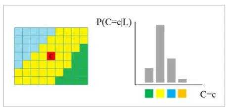
The size of the local context is important since it has to be big enough to describe the statistically probable shape of the object (e.g. a tendency that buildings have straight edges that separate them from the other ob-jects in the image), and small enough to not degrade the performance of the system, since the impact of the neighborhood decreases with the distance. Local context samples that we obtain by appearance-based segment classification are represented as a vector of discrete labels (encoded as integers) that correspond to the class labels of the adjacent segments. We do not incorporate into the sample the class label of the central segment, but we rather use it as a label of the sample. Our approach is similar but simpler then [25] where class probabilities were used as features. To accomplish the things stated in the second as-sumption, we need to show that we can learn to ap-proximate distribution P(C|L) from the local context samples. (An example of a distribution of the central segment class probability P(C|L) is given in Figure 4.). Since the smaller differences between features of samples do not impact the distribution P(C|L), our model allows for typical local context prototypes to be created. For this we use k-modes algorithm [14].

K-modes algorithm creates centroids that represent prototypes of the local contexts, so that the new sam-ples can be classified according to the most similar prototype.

When we determine the prototypes, we can calculate

P(C = c|L) for each prototype by calculating the fre-quency with which the number of samples that be-longs to a certain centroid and whose central segment class is equal to c appears in the total number of sam-ples that belong to that centroid. An exact number of prototypes cannot be determined analytically in ad-vance, but it can be assumed that each class will have a limited number of local contexts in which it appears in a training set. Training set is limited and a large number of prototypes should not be used since then the prototypes would be represented by a number of samples that is too small to later accurately approxi-mate P(C|L). In practice, we can determine the opti-mal number of prototypes by using cross-validation. Global context

The proposed model assumes that it is possible to describe and differentiate between different global image contexts, and that it is possible to approximate the distributions for each image class. Global image context can be described in many ways, for exam-ple as image gist [18], by a “bag of features” used for content-based image classification [22], through se-mantical features of a scene [18] or through features obtained on the level of image regions [9]. Images in the training set can then be divided into classes by unsupervised learning, and distributions P(C|L, G),

P(C|X, G) and P(C|G) can be approximated for each image class. Alternatively, it is possible to describe Figure 4

(7)

the global semantic context using basic appear-ance-based segment classification, and then create normalized histograms that represent the distribu-tion of classes in the images.

Model validation

We validated our proposed model on two image datasets: Stanford Background Dataset (SBD) [12] and FESB Mediterranian Landscape Image Data-set (FESB MLID) [10]. While validating our model on SBD dataset we used five-fold cross validation as in [12], [24] and [23], so that our results can be more comparable with the results of other researchers so that we can compare our classification results to theirs.

As a metric for the success of a given system we took a standard metric defined in previous works that dealt with similar problems and on similar datasets. The metric is expressed as a percentage of accurate-ly classified pixels on all of the images used in testing and validation phase, and we will refer to it as

classi-fication accuracy. This metric excludes all the pixels that are not labeled (i.e. that are typically labeled 0). The final expression is given in equation (12), where

real_class(p) denotes the real class of a pixel and

class(p) denotes the pixel class that is predicted by the model that is being tested:

�� |��|��|

|��|��| (12) (12)

where b1= real_class(p).

The systems compared were: [12], [24], [17], [23] and [8], and comparison for part of them can be found in [24]. Same as in our work, all of these systems were tested with the same protocol (5-fold cross-valida-tion) on SBD image dataset. The performance of our model, when using only the basic detection meth-od (boosted decision trees over uniform image seg-ments), i.e. no context information, was 67.0% on SBD dataset. However, if we added context information, the performance of our system increased to 73.6%. Although our model did not perform as well as other systems because we used relatively simple features

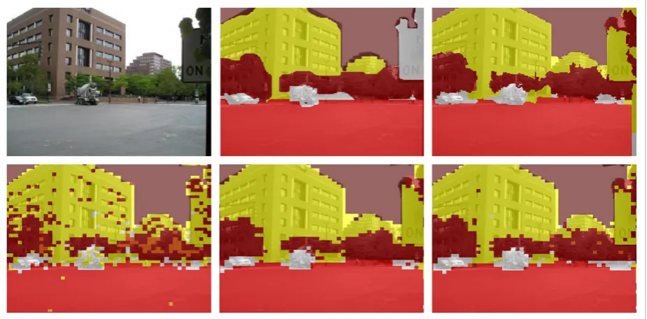
Figure 5

First row: original image from the SBD dataset, hand-labeled segmentation and classification, classification results obtained by NACC. Second row: based classification, context-based classification, combined appearance-based and context-appearance-based classification over uniform segments. This image was classified with 85% accuracy

(8)

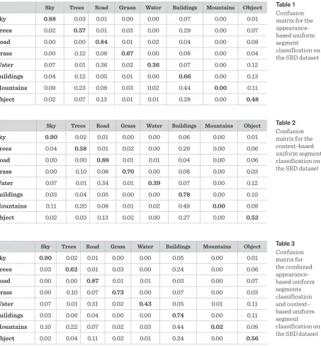
for appearance-based object classification, the in-crease in classification accuracy that happened after context was added to the model was the highest in our model. Figure 3 shows clasification results on one of the images from SBD dataset, while Tables 3, 1, 2 and 3 represent classification results obtained by our model on the SBD dataset. From these tables, we can point

Table 1 Confusion matrix for the appearance-based uniform segment classification on the SBD dataset

Table 2 Confusion matrix for the context-based uniform segment classification on the SBD dataset

Sky Trees Road Grass Water Buildings Mountains Object

Sky 0.88 0.03 0.01 0.00 0.00 0.07 0.00 0.01

Trees 0.02 0.57 0.01 0.03 0.00 0.29 0.00 0.07

Road 0.00 0.00 0.84 0.01 0.02 0.04 0.00 0.08

Grass 0.00 0.12 0.08 0.67 0.00 0.08 0.00 0.04

Water 0.07 0.01 0.36 0.02 0.36 0.07 0.00 0.12

Buildings 0.04 0.12 0.05 0.01 0.00 0.66 0.00 0.13

Mountains 0.09 0.23 0.08 0.03 0.02 0.44 0.00 0.11

Object 0.02 0.07 0.13 0.01 0.01 0.28 0.00 0.48

Sky 0.90 0.02 0.01 0.00 0.00 0.06 0.00 0.01

Trees 0.04 0.58 0.01 0.02 0.00 0.29 0.00 0.06

Road 0.00 0.00 0.88 0.01 0.01 0.04 0.00 0.06

Grass 0.00 0.10 0.08 0.70 0.00 0.08 0.00 0.03

Water 0.07 0.01 0.34 0.01 0.39 0.07 0.00 0.12

Buildings 0.03 0.04 0.05 0.00 0.00 0.78 0.00 0.10

Mountains 0.11 0.20 0.08 0.01 0.02 0.49 0.00 0.09

Object 0.02 0.03 0.13 0.02 0.00 0.27 0.00 0.52

out the mountains class that is certainly the most difficult to classify since it has fuzzy appearance but clear semantical meaning. This class is also weakly represented in the data set so it’s often confused with buildings, trees or sky. Adding contextual information can sometimes correct errors of appearance-based classification.

Table 3 Confusion matrix for the combined appearance-based uniform segments classification and context-based uniform segment classification on the SBD dataset

Sky 0.90 0.02 0.01 0.00 0.00 0.05 0.00 0.01

Trees 0.03 0.62 0.01 0.03 0.00 0.24 0.00 0.06

Road 0.00 0.00 0.87 0.01 0.01 0.03 0.00 0.07

Grass 0.00 0.10 0.07 0.73 0.00 0.07 0.00 0.03

Water 0.07 0.01 0.31 0.02 0.43 0.05 0.01 0.11

Buildings 0.03 0.06 0.04 0.00 0.00 0.74 0.00 0.11

Mountains 0.10 0.22 0.07 0.02 0.03 0.44 0.02 0.09

(9)

FESB MLID dataset is the subset of images ob-tained mostly from different wildfire surveillance cameras positioned in Dalmatia and Istria through the Croatian iForestFire (Intelligent Forest Fire Monitoring System) project, but it also containes images from [5] and [15]. At the time of writing of this article, the FESB MLID dataset is unpub-lished and not entirely completed and at the pres-ent time encompasses 300 images for the training stage, and 71 image for the testing stage of the im-age processing algorithms that use it. The dataset is labeled and encompasses 11 classes defined in [16]: smoke, clouds and fog, sun and light effects, sky, sea, distant landscape, rock, distant vegeta-tion, close vegetavegeta-tion, low vegetation and agricul-tural areas, and buildings and artificial objects. Unknown parts of the images are labeled as zero. Figure 5 shows classification results on one of the images from FESB MLID dataset. Tables 6, 7, 9 and

Table 4 Confusion matrix for the final superpixels classification on the SBD dataset

Sky 0.91 0.02 0.01 0.00 0.00 0.05 0.00 0.01

Trees 0.03 0.63 0.01 0.03 0.00 0.24 0.00 0.06

Road 0.00 0.00 0.88 0.01 0.01 0.03 0.00 0.07

Grass 0.00 0.10 0.07 0.73 0.00 0.07 0.00 0.03

Water 0.06 0.01 0.31 0.02 0.44 0.05 0.01 0.11

Buildings 0.03 0.05 0.04 0.00 0.00 0.76 0.00 0.11

Mountains 0.10 0.22 0.07 0.02 0.03 0.46 0.01 0.10

Object 0.02 0.04 0.11 0.01 0.01 0.24 0.00 0.57

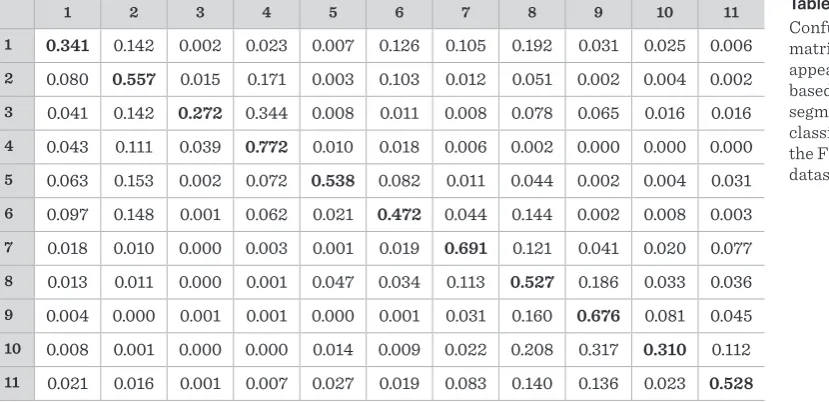
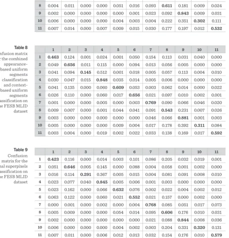
8 represent confusion matrices and the numbers written in bold represent the image classes in the following way: (1) smoke, (2) clouds and fog, (3) sun and light effects, (4) sky, (5) sea, (6) distant landscape, (7) rock, (8) distant vegetation, (9) close vegetation, (10) low vegetation and agricultural ar-eas and (11) buildings and artificial objects. From these tables we can point out smoke class that was central for this dataset. Based only on appearance, smoke is often confused equally with clouds and fog, distant landscape, rock and distant vegetation. By adding context to the classification of smoke we can see that the confusion with clouds and fog, dis-tant landscape and rock is lower, but the confusion with distant vegetation is higher. This higher con-fusion can be explained by the similar context for both smoke and distant vegetation in this dataset. Similar conclusions can be drawn for other classes where context is similar (e.g. sky and sun and light

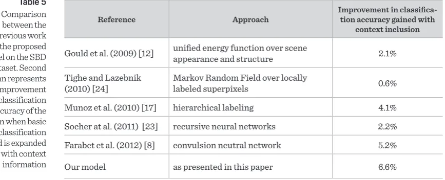
Table 5 Comparison between the previous work and the proposed model on the SBD dataset. Second column represents the improvement in classification accuracy of the system when basic classification method is expanded with context information

Reference Approach Improvement in classifica-tion accuracy gained with

context inclusion

Gould et al. (2009) [12] unified energy function over scene _{appearance and structure} 2.1%

Tighe and Lazebnik

(2010) [24] Markov Random Field over locally labeled superpixels 0.6% Munoz et al. (2010) [17] hierarchical labeling 4.1% Socher at al. (2011) [23] recursive neural networks 2.2% Farabet et al. (2012) [8] convulsion neutral network 5.2%

(10)

Figure 6

First row: original image from the FESB MLID dataset, hand-labeled segmentation and classification, classification results obtained by NACC. Second row: appearance-based classification, context-based classification, combined appearance-based and context-based classification over uniform segments. This image was classified with 94% accuracy

Table 6 Confusion matrix for the appearance-based uniform segments classification on the FESB MLID dataset

1 2 3 4 5 6 7 8 9 10 11

1 0.341 0.142 0.002 0.023 0.007 0.126 0.105 0.192 0.031 0.025 0.006

2 0.080 0.557 0.015 0.171 0.003 0.103 0.012 0.051 0.002 0.004 0.002

3 0.041 0.142 0.272 0.344 0.008 0.011 0.008 0.078 0.065 0.016 0.016

4 0.043 0.111 0.039 0.772 0.010 0.018 0.006 0.002 0.000 0.000 0.000

5 0.063 0.153 0.002 0.072 0.538 0.082 0.011 0.044 0.002 0.004 0.031

6 0.097 0.148 0.001 0.062 0.021 0.472 0.044 0.144 0.002 0.008 0.003

7 0.018 0.010 0.000 0.003 0.001 0.019 0.691 0.121 0.041 0.020 0.077

8 0.013 0.011 0.000 0.001 0.047 0.034 0.113 0.527 0.186 0.033 0.036

9 0.004 0.000 0.001 0.001 0.000 0.001 0.031 0.160 0.676 0.081 0.045

10 0.008 0.001 0.000 0.000 0.014 0.009 0.022 0.208 0.317 0.310 0.112

11 0.021 0.016 0.001 0.007 0.027 0.019 0.083 0.140 0.136 0.023 0.528 effects, sea and distant landscape, etc.). Table 4

shows the comparison between the previous work and the proposed model based on the results re-ported in referenced works. Since approaches and baselines in other works are very different, it can

(11)

1 2 3 4 5 6 7 8 9 10 11

1 0.405 0.122 0.000 0.015 0.002 0.095 0.091 0.220 0.034 0.016 0.001

2 0.049 0.641 0.004 0.145 0.001 0.083 0.008 0.063 0.004 0.003 0.000

3 0.015 0.134 0.263 0.368 0.005 0.017 0.005 0.086 0.091 0.007 0.010

4 0.023 0.079 0.038 0.841 0.004 0.006 0.005 0.003 0.001 0.000 0.000

5 0.023 0.156 0.000 0.063 0.610 0.085 0.002 0.036 0.012 0.002 0.012

6 0.059 0.132 0.000 0.066 0.018 0.532 0.027 0.164 0.001 0.001 0.000

7 0.000 0.002 0.000 0.002 0.000 0.003 0.764 0.092 0.059 0.019 0.058

8 0.004 0.011 0.000 0.000 0.051 0.016 0.093 0.611 0.181 0.009 0.024

9 0.002 0.000 0.000 0.000 0.000 0.001 0.023 0.092 0.843 0.009 0.031

10 0.006 0.000 0.000 0.000 0.004 0.003 0.004 0.222 0.351 0.302 0.111

11 0.007 0.014 0.000 0.007 0.009 0.015 0.030 0.177 0.197 0.012 0.532

Table 8 Confusion matrix

for the combined appearance-based uniform

segments classification and context-based uniform

segments classification on the FESB MLID dataset

1 2 3 4 5 6 7 8 9 10 11

1 0.463 0.124 0.001 0.024 0.001 0.050 0.154 0.113 0.031 0.040 0.000

2 0.049 0.656 0.011 0.115 0.000 0.094 0.013 0.056 0.005 0.000 0.000

3 0.041 0.094 0.145 0.512 0.001 0.018 0.005 0.057 0.113 0.004 0.010

4 0.030 0.047 0.015 0.848 0.035 0.014 0.005 0.006 0.000 0.000 0.000

5 0.041 0.135 0.000 0.060 0.609 0.053 0.003 0.062 0.014 0.000 0.022

6 0.026 0.110 0.000 0.060 0.017 0.656 0.021 0.097 0.010 0.002 0.001

7 0.001 0.000 0.000 0.005 0.000 0.003 0.769 0.090 0.066 0.046 0.020

8 0.009 0.007 0.000 0.001 0.044 0.041 0.091 0.543 0.231 0.007 0.026

9 0.003 0.000 0.000 0.000 0.000 0.000 0.046 0.066 0.881 0.001 0.003

10 0.005 0.000 0.000 0.000 0.009 0.004 0.017 0.178 0.392 0.311 0.084

11 0.003 0.004 0.000 0.019 0.002 0.022 0.033 0.138 0.169 0.017 0.592

Table 9 Confusion matrix for the final superpixels classification on the FESB MLID dataset

1 2 3 4 5 6 7 8 9 10 11

1 0.423 0.116 0.000 0.014 0.003 0.101 0.086 0.205 0.032 0.019 0.001

2 0.051 0.646 0.005 0.145 0.000 0.088 0.004 0.058 0.001 0.002 0.000

3 0.016 0.114 0.291 0.367 0.005 0.015 0.004 0.081 0.091 0.008 0.010

4 0.023 0.077 0.040 0.845 0.005 0.006 0.001 0.003 0.000 0.000 0.000

5 0.023 0.162 0.000 0.066 0.632 0.076 0.002 0.022 0.004 0.002 0.012

6 0.063 0.122 0.000 0.060 0.021 0.552 0.021 0.157 0.000 0.002 0.000

7 0.000 0.001 0.000 0.002 0.000 0.004 0.768 0.085 0.051 0.017 0.073

8 0.005 0.009 0.000 0.000 0.054 0.014 0.095 0.606 0.176 0.010 0.031

9 0.002 0.000 0.000 0.000 0.000 0.000 0.021 0.088 0.844 0.008 0.036

10 0.006 0.000 0.000 0.000 0.004 0.002 0.003 0.204 0.331 0.320 0.131

11 0.007 0.011 0.000 0.006 0.012 0.013 0.032 0.154 0.176 0.010 0.579 Table 7

Confusion matrix for the

(12)

Conclusion

In this work we presented a new model for non-para-metric context-based object classification. We val-idated the proposed model on SBD and FESB MLID datasets, and the results have shown that, when test-ed against other similar models, our model showtest-ed the greatest improvement in classification accura-cy when context was added to it (i.e. the strength of the context used in this model was greater that the strengths of the contexts used in previous works). Model validation also showed that the performance of our model is comparable to the best parametric systems for context-based object classification, but that it is also in direct dependence on the success of the basic appearance-based classifier. The proposed model allows the classification process to be inde-pendent of precise image segmentation, and it also enables deterministic process that unifies appear-ance-based and context-based classifications. In ad-dition, the proposed model also introduces a novel model for the description of a local context of a seg-ment by using uniform grid segseg-mentation of the im-age. This is achieved by the use of appearance-based classification results as local context description fea-tures, and by the adaptation of the k-modes algorithm to be able to classify those samples. Such a model al-lows the expansion of the existing system for the ap-pearance-based classification with the context-based classification, the precise determination of classifi-cation improvement when using context and the in-dependence of training appearance-based classifiers

and local context-based classifiers. The implementa-tion of the proposed system is modular, so it is possi-ble to change certain parts of it without them directly affecting the rest of the model.

In further work, we could include in our proposed model the use of global context, more sophisticated appearance-based features and classifiers, partial information about the shape of the objects obtained from superpixels and different uniform segmenta-tions of the image (e.g. log-polar description of local context [2]).

In addition to the described capabilities of the NACC model, non-parametric approach to appear-ance-based and context-based object classification still leaves much space for research. The non-para-metric approaches to object classification are rela-tively unexplored, so the model presented in this work could serve as the basis for research in non-paramet-ric use of contextual information.

Acknowledgements

This paper was largely based on the following PhD dissertation: Toma Rončević, “Nonparametric con-text based object classification in images”, University of Split, Faculty of Electrical Engineering, Mechan-ical Engineering and Naval Architecture, 2013. The authors would like to thank the anonymous reviewers for their constructive comments that helped improve this paper.

References

1. R. Achanta, A. Shaji, K. Smith, A. Lucchi, P. Fua, S. Süsstrunk. Slic superpixels. École Polytechnique Fédéral de Lausssanne (EPFL), Technical Report, 2010, 149300.

2. H. Araujo, J. M. Dias. An introduction to the log-polar mapping [image sampling]. In: Proceedings Second Workshop on Cybernetic Vision, 1996, 139-144 3. S. Ayache, G. Quénot, S. Satoh. Context-based

conceptu-al image indexing. In: Proceedings IEEE Internationconceptu-al Conference on Acoustics, Speech and Signal Processing (ICASSP), 2006, 2, 421-424. https://doi.org/10.1109/ icassp.2006.1660369

4. I. Biederman. Recognition-by-components: A theo-ry of human image understanding. Psychological Re-view, 1987, 94, 115-147. ttps://doi.org/10.1037/0033-295X.94.2.115

5. M. Bugarić, T. Jakovčević, D. Stipaničev. Adaptive esti-mation of visual smoke detection parameters based on spatial data and fire risk index. Computer Vision and Image Understanding, 2014, 118, 184–196. https://doi. org/10.1016/j.cviu.2013.10.003

(13)

So-Information Technology and Control 2017/1/46 98

ciety Conference on Computer Vision and Pattern Recognition, 2009, 1271-1278. https://doi.org/10.1109/ cvpr.2009.5206532

7. R. O. Duda, P. E. Hart, D. G. Stork. Pattern Classification, 2nd ed. Wiley-Interscience, 2000.

8. C. Farabet, C. Couprie, L. Najman, Y. LeCun. Scene pars-ing with multiscale feature learnpars-ing, purity trees, and optimal covers. ArXiv preprint arXiv:1202.2160, 2012. 9. L. Fei-Fei, P. Perona. A bayesian hierarchical model for

learning natural scene categories. In: IEEE Computer Society Conference on Computer Vision and Pattern Recognition (CVPR), 2005, 2, 524-531. https://doi. org/10.1109/cvpr.2005.16

10. FESB Mediterranian Landscape Image Dataset (FESB MLID). http://wildfire.fesb.hr/. Accessed on September 30, 2014.

11. Y. Freund, R. Schapire. A decision-theoretic generaliza-tion of on-line learning and an applicageneraliza-tion to boosting. In: Proceedings of the Second European Conference on Computational Learning Theory, 1995, 23-37. https:// doi.org/10.1007/3-540-59119-2_166

12. S. Gould, R. Fulton, D. Koller. Decomposing a scene into geometric and semantically consistent regions. In: IEEE 12th International Conference on Computer Vision, 2009, 1-8. https://doi.org/10.1109/iccv.2009.5459211 13. G. Heitz, D. Koller. Learning spatial context: Using

stuff to find things. In: Computer Vision-ECCV 2008, Springer, 2008, 30-43. https://doi.org/10.1007/978-3-540-88682-2_4

14. Z. Huang. Extensions to the k-means algorithm for clustering large data sets with categorical values. Data Mining and Knowledge Discovery, 1998, 2(3), 283-304. https://doi.org/10.1023/A:1009769707641

15. T. Jakovčević, D. Krstinić. Image and video databas-es. http://wildfire.fesb.hr/. Accessed on September 30, 2014.

16. T. Jakovčević. Wildfire-smoke detection based on visi-ble-specturm image analysis. PhD Thesis (in Croatian), University of Split, Faculty of Electrical Engineering, Mechanical Engineering and Naval Architecture, 2011. 17. D. Munoz, J. A. Bagnell, M. Hebert. Stacked hierarchical

labeling. In: Proceedings of the 11th European Conference on Computer vision: Part VI, Berlin, Heidelberg, 2010, 57-70. https://doi.org/10.1007/978-3-642-15567-3_5 18. A. Oliva, A. Torralba. Modeling the shape of the scene:

A holistic representation of the spatial envelope. Inter-national Journal of Computer Vision, 2001, 42(3), 145-175. https://doi.org/10.1023/A:1011139631724

19. G. T. Papadopoulos, C. Saathoff, H. J. Escalante, V. Mezaris, I. Kompatsiaris, M. G. Strintzis. A compar-ative study of object-level spatial context techniques for semantic image analysis. Computer Vision and Im-age Understanding, 2011, 115, 1288-1307. https://doi. org/10.1016/j.cviu.2011.05.005

20. T. Rončević, M. Braović, D. Stipaničev. Context-Based Natural Image Parsing: A Critical Survey. SoftCOM, 2011. 21. J. Shotton, M. Johnson, R. Cipolla. Semantic texton

forests for image categorization and segmentation. In: IEEE Conference on Computer Vision and Pattern Recognition (CVPR), 2008, 1-8. https://doi.org/10.1109/ cvpr.2008.4587503

22. J. Sivic, A. Zisserman. Video Google: A Text Retrieval Approach to Object Matching in Videos. In: Proceed-ings of the 9th IEEE International Conference on Com-puter Vision, Washington, DC, USA, 2003, 2, 1470-1477. https://doi.org/10.1109/ICCV.2003.1238663

23. R. Socher, C. C. Lin, A. Y. Ng, C. D. Manning. Parsing Nat-ural Scenes and NatNat-ural Language with Recursive NeNat-ural Networks. In: Proceedings of the 28th International Con-ference on Machine Learning (ICML), 2011, 2, 129-136. 24. J. Tighe, S. Lazebnik. Superparsing: scalable

nonpara-metric image parsing with superpixels. Computer Vi-sion-ECCV, 2010, 352-365.

25. Z. Tu, X. Bai. Auto-context and its application to high-level vision tasks and 3D brain image segmenta-tion. IEEE Transactions on Pattern Analysis and Ma-chine Intelligence (PAMI), 2010, 32, 1744-1757. https:// doi.org/10.1109/TPAMI.2009.186

26. M. Varma, A. Zisserman. Statistical approaches to ma-terial classification. In: Proceedings of Indian Confer-ence on Computer Vision, Graphics and Image Process-ing, Copehagen, Denmark, 2002, 167-172.

27. J. Verbeek, B. Triggs. Region classification with Mar-kov field aspect models. In: CVPR, 2007. https://doi. org/10.1109/cvpr.2007.383098

28. J. Winn, J. Shotton. The layout consistent random field for recognizing and segmenting partially occluded ob-jects. In: IEEE Computer Society Conference on Com-puter Vision and Pattern Recognition, 2006, 1, 37-44. https://doi.org/10.1109/cvpr.2006.305

29. W.-S. Zheng, S. Gong, T. Xiang. Quantifying contextual information for object detection. In: IEEE 12th Interna-tional Conference on Computer Vision, 2009, 932-939. 30. J. Zhu, S. Rosset, H. Zou, T. Hastie. Multi-class

(14)

Summary / Santrauka

Segmentation and classification of objects in images is one of the most important and yet one of the most com-plex problems in computer vision. In this work we propose a new model for natural image object classification using contextual information at the level of image segments. Context modeling is largely independent of ap-pearance-based classification and proposed model enables simple upgrade of existing systems with informa-tion from global and/or local context. Context modeling is based on non-parametric use of appearance-based classification results which is a novel approach compared to previous systems that model context on a limited number of rules expressed with a fixed set of parameters. Model implementation resulted in a system that, in our simulations, showed stable improvement of the appearance-based object classification.