Observer Based on Sliding Mode Control for Ship Dynamic Positioning

(1)

Observer Based on Sliding Mode Control for Ship

Dynamic Positioning

Dr. Diallo Thierno Mamadou Pathe

Pr. Diallo Saliou Kabi

Abstract – The ship dynamic positioning is a new

technology for positioning and orientation applied to the ship or floating platform, which can resist to the influence of offshore wind, wave, and flow by automatically keeping the setting position. The sliding mode is the way for simple and robust control for automatic systems. In most cases, the only available system variables are the input and output; it is necessary from those information’s, to reconstruct the state of the model to perform the control. In this paper we propose an observer based on sliding mode control for the ship dynamic positioning.

Keywords – Control, Dynamic Positioning, Observer, Ship

Model, Sliding Mode.

I. I

NTRODUCTION

Many methods of process control use the principle of state feedback (optimal control, decoupling, pole placement, etc.). As in most cases, the only available system variables are the input and output; it is necessary from such information, to reconstruct the state of the model to perform the control. A state reconstructor or estimator is a system (Fig. 1) having as inputs, the inputs and outputs of the real process and the output is an estimate of the state of the process.

Fig. 1. Principle of an observer

Under the assumption of linearity of the process model, the basic structure of the estimator is always the same, but its realization will depend on the chosen context: continuous or discrete, deterministic or stochastic. In the case where this model is a deterministic model, the state reconstructor will be called observer. In the case of noisy systems where random phenomena occur, it is called filter. The use of an observer can be seen in monitoring, diagnosis, and control.

A. Monitoring

Monitoring includes the measurement of the value of a particular parameter and also the follow-up into variations in its value (so as to allow the true value of the parameter to be controlled within a required range). Occasionally, monitoring may refer to the simple surveillance of a parameter without numerical values. The monitoring is the periodic oversight in the implementation of an activity, intervention, project or program. It seeks to establish if inputs, processes and outputs are proceeding according to

plan. It includes the regular collection and analysis of data to assist timely decision-making, ensure accountability and provide the basis for evaluations and learning. Monitoring is an internal function in any project or organization.

B. Diagnosis

Fault diagnosis involves different steps (detection, isolation, estimation) to provide increasing knowledge about the fault. The term diagnosis is commonly used when at least the first two tasks (detection, isolation) are accomplished. Fault diagnosis is based on available input/output signals of the process [1].

C. Control

The control system consists of a controlled equipment (system) and a controlling system. The controlled system is an independent, existing equipment, machine, which is the object of the control. The controlling system is a set of each equipments by which the control is done [2].

Automation or automatic control is the use of various control systems for operating equipment such as machinery, processes in factories, steering and stabilization of ships, aircraft and other applications with minimal or reduced human intervention.

In general indeed, due to sensor limitations (for cost reasons, technological constraints, etc.), the directly measured signals do not coincide with all signals characterizing the system behavior. Those signals of interest roughly include time-varying signals characterizing the system (state variables), constant ones

(parameters), and unmeasured external ones

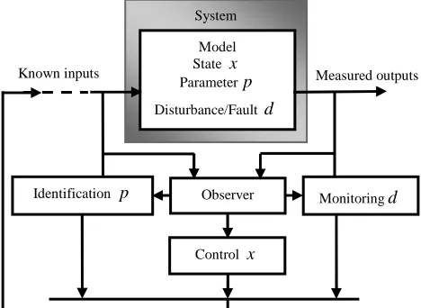
(disturbances). This need for internal information can be motivated by various purposes: modeling (identification), monitoring (fault detection), or driving (control) the system, all these being required for keeping a system under control, as summarized by figure (Fig. 2) hereafter.

Fig. 2. Observer as the heart of control systems

Process

State model x Outputs

Inputs _xˆ_{estimate of}_x

Reconstructor

System Model State x Parameterp Disturbance/Fault d

Observer _Monitoring_d

Control x Identification p

(2)

the heart of a general control problem [3].

The main techniques for synthesis of nonlinear observers are: observer’s canonical form, high gain observers, adaptive observer, observers by extended linearization, observers by optimization, and sliding mode observers. In this paper, a sliding mode observer is proposed for the ship dynamic positioning.

Sliding mode observer is a high performance state estimator which is well suited for uncertain nonlinear systems with partial state feedback [4], [5]. The sliding function of this observer is estimation error of the available output. The basic sliding mode observer consists of switching terms added to a conventional Luenberger observer [6].

II. M

ATHEMATICAL

M

ODEL OF THE

S

HIP FOR

DP

(D

YNAMIC

P

OSITIONING

)

The mathematical description of a system’s behavior is given by a model. When designing a control system, modern development in control theory has lead to an increased use of model knowledge. The best model is one that is accurate and descriptive enough, yet not too complex to implement or develop. Marine mechanics is a well-known field and a model is derived based on Newtonian and Lagrangian mechanics combined with a semi-empiric evaluation of hydrodynamic forces [7].

A. Formulation of Ship Model for DP

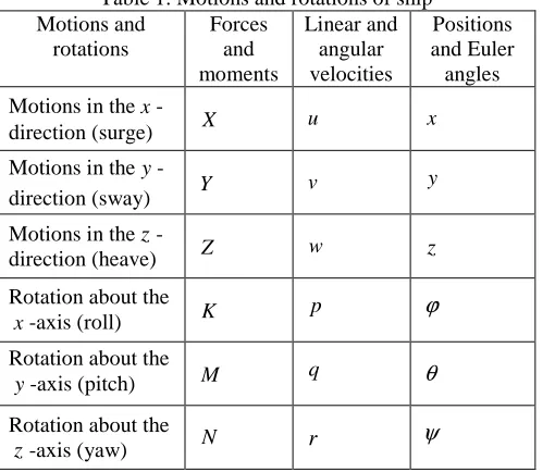
For marine vehicles, the six different motion components are conveniently defined as (Table 1): surge (the linear longitudinal “front/back” motion), sway (the linear lateral “side-to-side” motion), heave (the linear vertical “up/down” motion), roll (the rotation of a vessel about its longitudinal “front/back” axis), pitch (the rotation of a vessel about its transverse “side-to-side” axis), and yaw (the rotation of a vessel about its vertical axis).

Table 1. Motions and rotations of ship Motions and

rotations

Forces and moments

Linear and angular velocities

Positions and Euler angles Motions in the x

-direction (surge) X u x

Motions in they

-direction (sway) Y v

y

Motions in thez

-direction (heave) Z w z

Rotation about the

x -axis (roll) K p ϕ

Rotation about the

y -axis (pitch) M q θ

Rotation about the

z_{-axis (yaw)} N r ψ

For the analyses of the motion, it is convenient to define two coordinate frames as indicated in the figure (Fig. 3).

Fig. 3. Body fixed and earth fixed reference frame

The body fixed frame R_G=

{

G,X₀,Y₀,Z₀

}

is fixed to the vessel and the originG is usually chosen to be the

center of gravity of the vessel; R₀ =

{

O,X,Y,Z

}

is the earth-fixed reference frame. Based on the Euler’s theorem on rotation, the kinematic equations relating the body fixed reference frame to the earth-fixed reference frame can be expressed in vector for as:

( )

ηυ

ηɺ=J (1)

whereJ is the transformation matrix given by:

( )

  

 

  



 −

=

1 0 0

0 cos sin

0 sin cos

ψ ψ

η

J (2)

The vector υ=

[

u v w p q r

]

denotes the linear velocities in surge, sway and heave, and the angular velocities in roll, pitch and yaw, decomposed in the body fixed frame.

The position and orientation angles are gathered in a vector ηsuch that in the earth-fixed frame we have:

[

_x _y _z

_ϕ

_θ

_ψ

]

T

η

= (3)

The nonlinear six degrees-of-freedom body-fixed coupled equations of the motions in surge, sway, heave, roll, pitch and yaw are written as follows [7], [8], [9]:

( )

D

( )

G

( )

_thr env C

M

υ

ɺ+

υ

+

υ

+

η

=

τ

+

τ

(4) where M is the added mass due to the inertia of the surrounding fluid, D is the hydrodynamic damping matrix,

Cis the coriolis and centripetal matrix, Gis the vector of gravitational and buoyant forces and moments, τ_thrthe control forces, and τ_envthe environmental disturbances.

In dynamic positioning it has been adequate to regard the control objective as the three degree of freedom problem in the horizontal plane in surge, sway and yaw

0

G

0

Y

0

X 0

Z Pitch

Sway

Surge

Roll Heave

Yaw

Y

X Z

(3)

respectively. The coriolis and centrifugal matrices for the added mass and the rigid body can also be crossed out of the equation because in low speed applications, quadratic velocity terms are negligible. The gravitational forces are not included either due to the inexistence of forces coupled to the dynamics. The dynamic equation (4) is therefore simplified to:

( )

thr env

D

Mυɺ+ υυ=τ +τ (5)

with η =

[

x y ψ

]

Tand υ=

[

u v r

]

By taking τthr+τenv=τ, the equation (5) becomes:

( )

υυ τ

υ+D =

Mɺ (6)

So the reduced equations of motion of Ship dynamic positioning (DP) in surge, sway and yaw can be expressed as follows [12]:

( )

   = = + υ η η τ υ υ J D M ɺ ɺ (7)

B. State Space Representation of the Ship Model

From the successive derivative of ηand the change of variablesx1=η, x2=xɺ1and x3 =xɺ2the system (7) can be

represented in state space as:

       + = + − + + = = = − − U B f B x A B B A x B B A x x x x x 2 2 2 1 3 1 3 3 2 2 1 ] [ ] [ ɺ ɺ ɺ τɺ ɺ ɺ ɺ (8)

withA=[Jɺ−JM−1D]J−1, B=JM−1=B₂, τɺ=U,

2 1 3

1

2 [A BB ]x [A BB A]x

f = + ɺ − + ɺ− ɺ − ,x₁=η =[x,y,

ψ

]T,

1

2 x

x = ɺ , andx₃ =xɺ₂.

By choosing the new change of variablesx=X₁,y=Y₁, andψ =Z₁with their successive corresponding derivatives

2

1 X

Xɺ = , Xɺ₂=X₃, Yɺ₁=Y₂, Yɺ₂ =Y₃, Zɺ₁=Z₂, and

3

2 Z

Zɺ = , the system (8) becomes:

( ) ( )

                + =                     =                     =           X U X B X f Z Y X Z Y X Z Y X Z Y X Z Y X 2 2 3 3 3 3 3 3 2 2 2 2 2 2 1 1 1 ) ( ɺ ɺ ɺ ɺ ɺ ɺ ɺ ɺ ɺ (9)

[

]

T

Z Y

X f f

f X

f2( )= 2 2 2

III. S

LIDING

M

ODE

O

BSERVER

A

PPLIED TO THE

S

HIP

Several structures of observers are possible for the estimation of the state of the system model [10], [11], [12], [13]. In this part, the so called sliding mode triangular observer is proposed.

A.

Lemma

For the system model defined in (9), the sliding mode observer which makes the observing errors tend to zeros in finite time can be written as:

(

)

(

)

(

)

(

)

(

)

(

)

( ) ( )

(

)

(

)

                             − − − Λ + + =                       − − − Λ +           =                       − − − Λ +           =             3 3 3 3 3 3 3 2 2 3 3 3 2 2 2 2 2 2 2 3 3 3 2 2 2 1 1 1 1 1 1 1 2 2 2 1 1 1 ˆ ˆ ˆ ) ( ˆ ˆ ˆ ˆ ˆ ˆ ˆ ˆ ˆ ˆ ˆ ˆ ˆ ˆ ˆ ˆ ˆ ˆ ˆ ˆ ˆ Z Z sign Y Y sign X X sign X U X B X f Z Y X Z Z sign Y Y sign X X sign Z Y X Z Y X Z Z sign Y Y sign X X sign Z Y X Z Y X ɺ ɺ ɺ ɺ ɺ ɺ ɺ ɺ ɺ (10) with           Λ Λ Λ = Λ iZ iY iX i 0 0 0 0 0 0

, i=1,2,3

B. Proof

From the system (10), the dynamic of the observer error

i i

iR R R

E = − ˆ (with E₁_R =R₁−Rˆ₁, R₁=R₁,

(

1 1

)

) 1 ( ˆ ˆ − − − − Λ +

= i i R i i

i R signR R

R , i=2,3, and

Z Y X

R= , , ) is:

(

)

(

)

(

)

(

)

(

)

(

)

(

)

(

)

(

)

                 − Λ − − = − Λ − = − Λ − = − Λ − − = − Λ − = − Λ − = − Λ − − = − Λ − = − Λ − = 3 3 3 2 2 3 2 2 2 3 2 1 1 1 2 1 3 3 3 2 2 3 2 2 2 3 2 1 1 1 2 1 3 3 3 2 2 3 2 2 2 3 2 1 1 1 2 1 ˆ ) ( ) ( ˆ ˆ ˆ ) ( ) ( ˆ ˆ ˆ ) ( ) ( ˆ ˆ Z Z sign X f X f E Z Z sign E E Z Z sign E E Y Y sign X f X f E Y Y sign E E Y Y sign E E X X sign X f X f E X X sign E E X X sign E E Z Z Z Z Z Z Z Z Z Z Y Y Y Y Y Y Y Y Y Y X X X X X X X X X X ɺ ɺ ɺ ɺ ɺ ɺ ɺ ɺ ɺ (11)

Step1: For the convergence of E1_Rin finite time we

consider a Lyapunov functionV₁=E₁2_R/2

(

)

(

2 1 1 1

)

1 1 1

1 E E E E signR Rˆ

Vɺ = _Rɺ _R= _R _R−Λ_R −

max 2 1

1 0 R E R

(4)

ofE1_Rafter a finite timet1toward zero.

After t₁, the state reaches the sliding surface and on this

surface, we have E₁_R=Eɺ₁_R =0 then we have: R₂=R₂. Step 2: while respecting the condition of convergence of the first step; let’s show the convergence of E2_Rin

finite time.

By replacing R₂ =R₂ one gets: Eɺ₂_R=E₃_R−

( )

R Rsign E2 2

Λ .

Let choose the Lyapunov function V₂=

(

E₁2_R+E₂2_R

)

/2 one has after t₁, E1R =0from where:

( )

(

R R R

)

R R

RE E E signE

E

Vɺ₂= ₂ ɺ₂ = ₂ ₃ −Λ₂ ₂

max 3 2

2 0 R E R

Vɺ ≤ ⇔Λ >

By choosing Λ2R > E3R_maxwe obtain the convergence of E2_Rafter a finite time t2 >t1 toward zero.

After t₂, the state reaches the sliding surface and on

this surface, we have E₂_R=Eɺ₂_R=0from where we got:

3

3 R

R = .

Step 3: By respecting the conditions of convergence of the first and the second step; let show the convergence of

R

E3 in finite time.

While replacing R₂=R₂, R₃=R₃one gets:

( )

R R

R signE

Eɺ₃ =−Λ₃ ₃

We choose the Lyapunov function:

(

₁2 ₂2 ₃2

)

/2

3 ER E R E R

V = + + , after t₂, E1R =E2R =0 from where:

( )

(

R R

)

R R

RE E signE

E

Vɺ₃ = ₃ ɺ₃ = ₃ −Λ₃ ₃

0

0 ₃

3< ⇔Λ R>

Vɺ

By choosing Λ₃_Rin the vicinity of zero we obtain the convergence of E3_Rafter t3>t2.

IV. S

LIDING

M

ODE

C

ONTROLLER

A

PPLIED TO THE

S

HIP

In the precedent section, we have show the convergence of observer error that means after a finite time we have:

i

i R

R = ˆ . Now, let take the dynamic tracking error ri

i

iR R R

e = ˆ − whereR_riis the desired trajectory. By taking e1=

[

e1_X e1_Y e1_Z

]

T, e2 =eɺ1,

[

]

T

Z Y

X e e

e

eɺ1= 2 2 2 , and

[

]

T Z Y

X e e

e e

e3 =ɺ2 = 3 3 3

we can define the sliding surface as: σ =e3+K

[

e1 e2

]

T

A. Theorem

For system model (10), the sliding mode controller which makes the tracking errors tend asymptotically to zeros in finite time is:

r eq U

U

U= + (12)

where U_eq=−B₂−1

β

is the equivalent control, and )

(

1 2 signσ

B Ur

−

= is the robust control term with

[

]

(

)

(

)

         − − − Λ +           − + = 3 3 3 3 3 3 3 2 2 2 2 3 2 ˆ ˆ ˆ ) ( Z Z sign Y Y sign X X sign Z Y X X f e e K r r r T ɺ ɺ ɺ β .

B. Proof

Step 1: The equivalent control law. On the sliding surface we have:

( ) ( )

X,t =σ X,t =0

σ ɺ

The first derivative with respect to t of σ is done:

( )

[

]

[

]

[

]

[

]

T

[

]

T

r r r T T T r r r T T Z Y X e e K Z Y X Z Y X e e K Z Z Y Y X X e e K e e e e e K e t X 3 2 3 3 3 3 3 3 3 2 3 3 3 3 3 3 3 2 3 3 3 3 2 3 ˆ ˆ ˆ ˆ ˆ ˆ , + −     = +     ₋ ₋ ₋ = + =       + = ɺ ɺ ɺ ɺ ɺ ɺ ɺ ɺ ɺ ɺ ɺ ɺ ɺ ɺ ɺ ɺ ɺ σ

( )

      −           =     ⇒ = 3 2 3 3 3 3 3

3 ˆ ˆ

ˆ 0 , e e K Z Y X Z Y X t X r r r T ɺ ɺ ɺ ɺ ɺ ɺ ɺ σ

( ) ( )

(

)

(

)

         − − − Λ + + = 3 3 3 3 3 3 3 2 2 ˆ ˆ ˆ ) ( Z Z sign Y Y sign X X sign X U X B X f _eq

( )

X B

( )

X

β

U_eq =− ₂−1

⇒ with

(

)

(

)

(

)

         −       +           − − − Λ + = 3 3 3 3 2 3 3 3 3 3 3 3 2 ˆ ˆ ˆ ) ( r r r Z Y X e e K Z Z sign Y Y sign X X sign X f ɺ ɺ ɺ β

Step 2: The robust control law. Let consider the candidate Lyapunov function V :

σ σ σ σ σ σ σ

σT Vɺ ɺT Tɺ Tɺ

V =( )/2⇒ =( + )/2=

[

]

              + −     = 3 2 3 3 3 3 3

3 ˆ ˆ

ˆ e e K Z Y X Z Y X

V _r _r _r T

T

T ɺ ɺ ɺ _ɺ _ɺ _ɺ

(5)

( )

(

)

(

)

(

)

    

    

 

    

    

 

      +   

 

  

  −

   

 

   

 

   

 

   

 

− −

− Λ

+ + +

=

3 2

3 3 3

3 3

3 2

2

ˆ ˆ

ˆ

e e K

Z Y X

Z Z sign

Y Y sign

X X sign

U U X B X f

r r r

r eq

T

ɺ ɺ ɺ σ

Replacing U_eqby its value in the precedent equation

we gotVɺ=

σ

T

(

B₂

( )

X U_r

)

; assumingU_r =−B₂−1sign(σ), the function Vɺ=−

σ

Tsign(

σ

)≤0

.

V. S

IMULATION

R

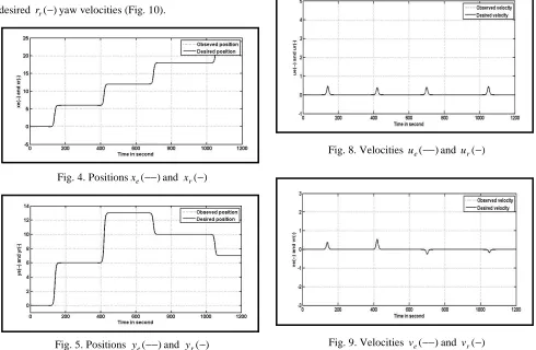
ESULTS

The numerical parameters of the model, the desired positions, linear velocities, angular velocity, and the values of H and K can be founds in our previous work [14]. The values ofΛ₁=0 I.9 ₃, Λ₂ =0 I.7 ₃,

Λ

₃

=

0 I

.

1

₃, where I is the identity matrix. The following figures ₃

shows respectively the observed xe(−−), ye(−−) and the desired x_r(−), y_r(−) positions (Fig. 4, Fig. 5); the observed ψe(−−)and the desired ψr(−)yaw angles (Fig. 6); the observed positiony in function of _e x (Fig. 7); the _e

observed ue(−−),

v

e

(

−−

)

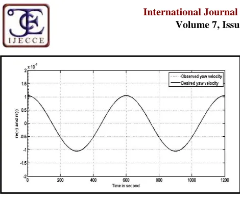
and desired ur(−), vr(−) velocities (Fig. 8, Fig. 9); the observed re(−−)and the desired r_r(−)yaw velocities (Fig. 10).

Fig. 4. Positionsxe(−−)and xr(−)

Fig. 5. Positions y_e(−−)and y_r(−)

Fig. 6. Yaw angles ψ_e(−−)and ψ_r(−)

Fig. 7. Position y in function of _e x _e

Fig. 8. Velocities u_e(−−)and u_r(−)

(6)

VI. C

ONCLUSION

In this work, we had studied the dynamic positioning of the ship by considering the uncertainties of the measures. For the reconstruction of the unmeasured states of the ship model, the sliding mode triangular observer is used. The simulations results show the good performance of the used techniques for our applications.

R

EFERENCES

[1] Mogens Blanke. Blanke, “Enhanced Maritime Safety Through

Diagnosis and Fault Tolerant Control”, Proc. IFAC conference

CAMS'2001, 2001.

[2] Ildiko Mako, “Fundamentals of Automation”, Machine Tool Department , University of Miskolc. 1997.

[3] Gildas Besancon, “Observer Design for Nonlinear System”, A. Loria et al. (Eds.): Advanced topics in Control Systems Theory, LNCIS 328, PP. 61-89, Springer, 2006.

[4] Vadim I. Utkin, “Sliding modes in control and optimization”, Springer-Verlag, 1992.

[5] Moura J T, Elmali H, et al, “Sliding mode control with sliding

perturbation observer”, J Dynam System, Measurement Control,

Trans ASME 1997; 119(4): 657-665.

[6] L. Jiang, Q. H. Wu, C. Zhang, and X. X. Zhou, “Observer-based

nonlinear control of synchronous generators with perturbation estimation”, Electrical Power and Energy Systems 23 (2001)

359-367.

[7] Rajesh Kumar Verma, “Dynamic Positioning of Ship using

Direct Model Reference Adaptive Control”, Thesis of College of

Graduate Studies Texas A&M University-Kingsville, 2004. [8] Zhang Cheng-Du, Wang Xi-Huai, Xiao Jian-Mei, “Ship

Dynamic Positioning System based on Backstepping Control”,

Journal of Theoretical and Applied Information Technology, 10th May 2013. Vol. 51 No.1, pp 129-136.

[9] Wen-Jer Chang, Guo-Chang Cheng, and Yi-Lin Yeh, “Fuzzy

Control of Dynamic Positionning Systems for Ships”, Journal of

Marine Science and Technology, Vol. 10, No. 1, pp. 47 – 53, 2002.

[10] Thor I. Fossen and Tristan Perez, “Kalman Filtering for

Positioning and Heading Control of Ships and Offshore Rigs”,

IEEE Control Systems Magazine, 2009.

[11] A. Mehmood, S. Laghrouche and M. El Bagdouri, “Position

tracking of the VGT Single Acting Pneumatic Actuator with 2nd order SMC and Backstepping Control Techniques”, 12th IEEE

Workshop on Variable Structure Systems, VSS’12, January 12-14, Mumbai, 2012.

[12] Liu Furong, Chen Hui, Gao Haibo, “Application of Moving

Horizon Filter for Dynamic Positioning Ship”, Journal of Wuhan

University of Technology. 2010; .32(12): 117-120.

[13] Manuel Jimenez-Lizárraga, Michael Basin, Celeste Rodriguez, Pablo Rodriguez, “HOSM Observer for Robust Output Regulator

in Uncertain Nonlinear Polynomial Systems”, 12th IEEE

Workshop on Variable Structure Systems, VSS’12, January 12-14, Mumbai, 2012.

[14] Diallo Thierno Mamadou Pathe, Li Hongsheng, Bian Guangrong, “Switching Surface Design for Nonlinear Systems:

the Ship Dynamic Positioning”, TELKOMNIKA (2013) 11(4),

1801- 1808.

A

UTHOR

’

S

P

ROFILE

Diallo Thierno Mamadou Pathe, native of Guinea was

born in 1976. He received the Bachelor degree of Physics in 2002 at the University Mohamed 1er Oujda, the Master degree of Automation and Information Processing in 2004 at the University Sidi Mohamed Ben Abdallah Fes (Morocco), and the Doctor degree of Engineering in Mechanical Manufacture and Automation in 2014 at Wuhan University of Technology (China).

In Guinea at the Centre Universitaire de Kindia he is a Lecturer since 2007, and 209-2010 Head of Division of Statistics, Documentation and Publication. June and July 2013 a Math’s lecturer at Wuhan University, China. He is currently an Assistant Professor. His research interests are control theories, signal analysis and information processing.

Dr. Diallo has been awarded by Wuhan University of Technology in 2013-2014 for the thesis “Digital Maintenance and Training of Digital Manufacturing” granted as the Outstanding Thesis Award for postgraduate students.

Diallo Saliou Kabi, native of Guinea was born in 1950.