Precision spray modeling using image processing and artificial
neural network
Amir Azizpanah
1, Ali Rajabipour
1*, Reza Alimardani
1, Kamran Kheiralipour
2,
Vahid Mohammadi
3(1. Department of Agricultural Machinery, University of Tehran, Karaj, Iran;
2.Mechanical Engineering of Biosystems Department, Ilam University, Ilam, Iran;
3.Department of Biosystems Engineering, Shahrekord University, Shahrekord, Iran.)
Abstract: This study employed artificial neural network method for predicting the sprayer drift under different conditions using image processing technique. A wind tunnel was used for providing air flow in different velocities. Water Sensitive Paper (WSP) was used to absorb spray droplets and an automatic algorithm processed the images of WSPs for measuring droplet properties including volume median diameter (Dv0.5) and Surface Coverage Percent (SCP). Four Levenberg-Marqurdt models were developed to correlate the sprayer drift (output parameter) to the input parameters (height, pressure, wind velocity and Dv0.5). The ANN models were capable of predicting the output variables in different conditions of spraying with a high performance. Both models predicted the output variables with R2 values higher than 0.96 indicating the accuracy of the selected networks. Therefore, the developed predictor models can be used in precision agriculture for decreasing spray costs and losses and also environmental contamination.
Keywords: sprayer, drift, image processing, artificial neural network.
Citation: Azizpanah, A., A. Rajabipour, R. Alimardani, K. Kheiralipour, and V. Mohammadi. 2015. Precision spray modeling using image processing and artificial neural network. Agric Eng Int: CIGR Journal, 17(2):65-74.
1 Introduction
1One of the seminal agents of environment’s
pollution is pesticide drift during agricultural operations
(Gil and Sinfort, 2005). The effective factors on spray
drift are the technique of spray application, canopy
properties, meteorological conditions, and
physicochemical properties of the spray liquid (De
Schampheleire et al., 2008). In recent years, many studies
have been performed to reduce the spray drift and
optimize the spray deposition (Jamar et al., 2010; Wolf
and Gardisser, 2014).
Industry, technology, education, and research are
being employed to address these concerns. Hence, several
standards and protocols including laboratory tests,
Received date: 2015-03-04 Accepted date: 2015-04-08 *Corresponding author: Ali Rajabipour. Department of Agricultural Machinery, University of Tehran, Karaj, Iran.Tel: +98-2612801011, Fax: +98-2612808138, Email: [email protected].
modeling, and under field condition tests are used to
evaluate sprays (Fritzet al., 2012). Using the mentioned
methods and protocols, researchers have studied spray
flow (Deleleet al., 2005; Endalew et al., 2010; Endalew et
al., 2010), dispersion of droplets (García-Santos et al.,
2011; Han et al., 2014), roll and pitch angles (Khot et al.,
2008), spray characteristics (Guler et al., 2006; Hewitt et
al., 2009; Jamar et al. 2010), drift risk (Balsari et al., 2007;
Qi et al., 2008), and canopy size (Escolà et al., 2013).
However, spray drift profusely is influenced by some
other factors such as equipment, application technique,
spray properties, operator skills, and environmental
conditions (Gilet al., 2014).
Therefore, the main reason of studies in this field is
to determine the most important factors and appropriate
measures for minimizing the drawbacks of spray
applications (Baetenset al., 2009). Different analytical,
numerical and predictive models have been used to
66 March, 2015 AgricEngInt: CIGR Journal Open access at http://www.cigrjournal.org Vol. 17, No. 2
virtual environment based on the real data of equipment,
weather conditions and spray characteristics (Baetenset
al., 2007; Bartzanas et al., 2013; Endalew et al., 2010;
Kennedy et al., 2012; Lebeau et al., 2011). However, just
in few studies Artificial Neural Networks (ANN)
technique for predicting spray process characteristics has
been developed. Pandaet al. (2001), studied the influence
of process parameters, drying conditions, impact
velocities and physical properties of sprayed solutions on
the kinetics of granulation and on the morphology of the
end product. They modeled the droplet deposition
behavior on a single particle in fluidized bed spray
granulation process using ANN led to useful results in
understanding the growth kinetics in spray-coating
process (Pandaet al., 2001). Krishnaswamy and Krishnan
(2002), predicted the nozzle wear rates for four fan
nozzles by using neural network technique and compared
the results with the regression technique. In another study,
a precision herbicide-spraying system was developed for
real-time image collection and processing, weed
identification, mapping of weed density, and sprayer
control (Yanget al., 2003). Heinleinet al. (2007), fitted
neural network models to the experimental data for
mapping the structure of a liquid spray system along the
spray cone. They reported that the general trends could
not be well predicted by the ANN models and they
concluded that it was due to unsteady spray conditions or
incomplete atomization (Heinleinet al., 2007).
In the current study, spray drift was investigated using
a wind tunnel. For this aim, the droplet diameter and drift
were measured by image processing technique and
predicted by artificial neural network. Also various
conditions including different wind speed, spraying
height and pressure were considered.
2 Materials and methods
The research was conducted at Mechanical
Engineering of Biosystems Department, Ilam University,
Ilam, Iran in October, 2014.
2.1 Experimental station and conditions
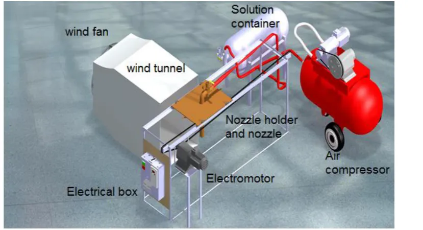
As the Figure 1 shows, a setup was used including
wind tunnel, sprayer system and mobile parts. The setup
was implemented on the ground. For stimulating the
tractor movement, a DC electromotor was used to power
the mobile parts. An air compressor provided various
spray pressures. A plate was used to hold the nozzle and a
rail was provided to support and facilitate its automatic
motion. The spraying liquid, water, was supplied in a tank
under the pressure of an air compressor.
A wind tunnel was set for providing air flow in
velocities of 0, 4, 8 and 12 km/h. At the entrance of wind
tunnel, an anemometer (AM-4206, Lutron, Taiwan) was
used for monitoring the air velocity. The spray pressure
was evaluated with a calibrated gauge that it was
connected to a capillary before the nozzle. The
experiments were performed for three different pressures
of 3, 4, and 5 bar. Temperature and moisture were
monitored using a digital thermometer (TM-917, Lutron,
Taiwan) and a hygrometer (HT-3015, Lutron, Taiwan),
respectively. Also the setup had an electrical box
including start and stop keys and a contactor for
switching the power.
For all of the experiments, an 11003 flat fan nozzle
(TeeJet, US) was used. Parameters of nozzle operation
were opted based on desired field application rates, plant
and products limitations and management practices.
Three spraying heights of 35, 50, and 65 cm were chosen
as the distance between the nozzle’s orifice and the
ground.
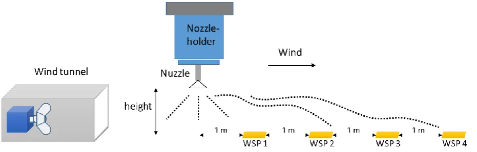
In order to provide high quality data, water sensitive
paper (WSP) was utilized for absorbing the spray droplets.
WSPs were situated in the positions of 1, 2, 3, and 4 m far
from the nozzle orifice (Figure 2). All of the experiments
were replicated three times.
2.2Image Acquisition and Processing
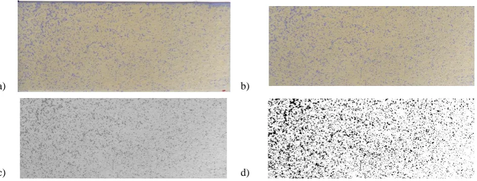
Images of WSPs were scanned by a photographic
scanner (CanoScanLiDe 110, Vietnam) to be processed.
Figure 3a indicates the WSP after absorbing water. As the
figure shows, the yellow paper has blue spots as droplets.
An automatic algorithm was developed in MATLAB
2010a software (The Mathworks Inc., USA) for images
processing. In the first step, images were imported to the
software and borders and interrupted edges were removed
(Figure 3b). Then, the red channels of the images were
obtained from RGB images (Figure 3c). After this, the
images were converted to binary images (Figure 3d).
The number of spray droplets were figured out and the
image of each droplet were separated in a special name.
After calculating area and equivalent diameter of droplets,
the surface coverage percent (SCP) was computed for
each place, e.g. SCP1, SCP2, SCP3 and SCP4
respectively for 1, 2, 3 and 4 m horizontal distance from
the nozzle.
68 March, 2015 AgricEngInt: CIGR Journal Open access at http://www.cigrjournal.org Vol. 17, No. 2
Then, the algorithm classified the droplets into five
different groups depending on the diameter of the spots.
After multiplying each diameter group in corresponding
coefficients (Nuyttenset al., 2007), the Volume Median
Diameter (VMD, Dv0.5), a diameter which smaller
droplets from that constitute 50 % of the total droplet
volumes, 10th and 90th percentile (Dv0.1 and Dv0.9) of
volume diameter and Relative Span Factor (RSF) were
calculated. For calculating these factors, first droplets
scattered on WSPs are arranged in order of droplets sizes.
Then, volumetric diameter and mean diameter of each
group are determined. VMD is the diameter that divides
all diameters into equal groups. Droplet size and
spectrum have been documented as the most influential
factor on drift (Wolf and Minihan, 2001). This variable is
expressed in microns and usually drift potential is
identified as the number of droplets smaller than a special
amount in microns. This variable can be used to
determine some valuable statistics including the percent
coverage, the spray deposition rate, droplet size
uniformity, drift profile, and swath pattern width (Wolfet
al., 2000). In addition, RSF and drift was calculated as
following (Nuyttenset al., 2007):
RSF = (Dv0.9 - Dv0.1)/ Dv0.5 (1)
Drift = SC1+SC2+SC3+SC4 (2)
2.3 Data Analysis
To predict the drift and VMD data, artificial neural
network (ANN) method was used. Thus, ANN technique
was employed to describe the relationships among
operating conditions of spraying pressure, wind velocity,
nozzle height, and RSF to associate them with drift. The
information about inputs and outputs of the models have
been presented in Table 1.
Table 1 The inputs and target variables of neural
networks
No.
Inputs
No. of neurons of input layer
Output
Net. 1 Pressure, Wind Velocity, Height
3
VMD Net. 2 Height, Wind Velocity,
RSF, VMD
11
Drift
The Levenberg-Marqurdt model was used for
training the network and the transfer functions of ‘tansig’ and ‘purelin’ were chosen for hidden and output layers,
respectively. All data sets were divided into three groups,
randomly: 70% for training the networks, 15% for
validation of the networks and the last 15% for testing the
networks. For sophisticated and non-linear relationships
appropriate number of hidden neurons is necessary to
correctly approximate the desired input-output
relationships (Safa and Samarasinghe, 2013). Therefore,
a) b)
c) d)
Figure 3 Image analysis, a) the original image b) trimmed image c) obtained red channel image and d) binary
many various types of network topologies were tested to
achieve the best predicting networks. One hidden layer
was considered and the number of its neurons was
changed to find the best model. A range of 3-20 neurons
were tested in the hidden layer. MATLAB 2010a (The
Mathworks Inc. USA) was used for designing and
running of all ANN models.
Many various neural networks were developed and
the optimum values of network’s performance were
obtained by trial and error. In order to estimate the
performance of trained networks, three factors including
mean square error (MSE) of validation data, correlation (r)
of test data, and coefficient of determination (R2) for
prediction of all data were used.
3 Results and discussion
Different types of neural networks topologies were
developed to model the relationships between the input
and output variables to produce models for predicting the
volumetric median diameter and drift phenomenon. The
performance of ANNs was evaluated using the mean
square error (MSE) of validation data, correlation (r) of
test data and R-square of prediction of all data. Tables 2
and Table 3 provide an overview of performance of the
neural networks for the best cases of topology for
predicting VMD and drift, respectively.
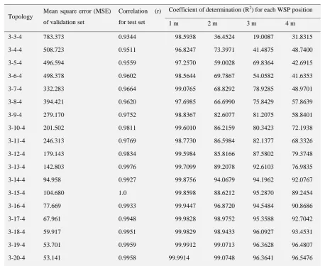
The best topology for predicting the VMD at each
distance was 3-20-4 that 3 is the number of input data
(pressure, wind velocity and height), 20 is the number of
neurons in hidden layer and 4 stands for the number of
output data (VMD at 1, 2, 3, and 4 m distance from
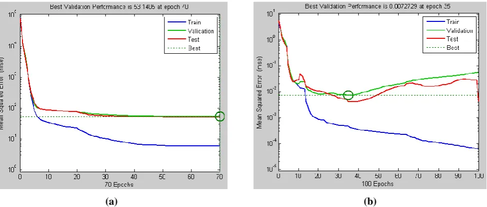
nozzle). The mean square error (MSE, Figure4a) of whole
validation set was 53.141.The correlation (r) for whole
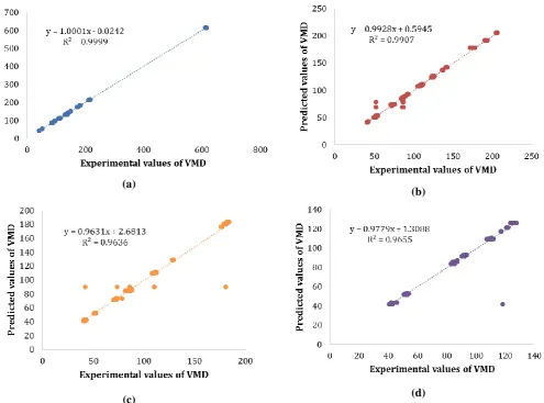
test set was obtained as 0.9958. The coefficient of
determination (R2) for predicting VMD in each WSP
position, i.e. 1, 2, 3 and 4 m, was 99.99%, 99.07%, 96.36%
and 96.55%, respectively (Figure5).
Table 2Performance of ANN model to predict VMD for different positions of WSPs
Topology Mean square error (MSE) of validation set
Correlation (r) for test set
Coefficient of determination (R2) for each WSP position
1 m 2 m 3 m 4 m
June, 2015 AgricEngInt: CIGR Journal Open access at http://www.cigrjournal.org Vol. 17, No. 2 70
According to Table 3, the best topology for predicting
the drift was gained with 11-9-1 structure. Eleven is the
number of input data (height, wind velocity, RSF at each
situation and VMD at each situation), 9 is the number of
neurons in hidden layer and 1 is the number of output
data (drift, D). In Figure 4b, the mean square error (MSE)
of validation set was presented as 0.0073.The correlation
(r) for test set of the model was 0.999. The coefficient of
determination (R2) was 99.81 % (Figure6).
Table 3Performance of ANN models to predict drift
Topology Mean square error (MSE) of validation set
Correlation (r) for test set
Coefficient of determination (R2) for drift
11-3-1 0.0141 0.9918 98.9805
11-4-1 0.258 0.9932 98.6601
11-5-1 0.0101 0.9971 99.6048
11-6-1 0.0226 0.9980 99.4143
11-7-1 0.0349 0.9975 97.7931
11-8-1 0.0273 0.9960 99.1060
11-9-1 0.0073 0.9987 99.8126
11-10-1 0.0112 0.9862 99.1702
11-11-1 0.0448 0.9966 99.1022
11-12-1 0.0144 0.9897 99.2980
11-13-1 0.0217 0.9225 96.0021
11-14-1 0.0149 0.9934 99.4621
11-15-1 0.0146 0.9984 99.7124
11-16-1 0.0126 0.9983 99.7186
11-17-1 0.0265 0.9973 99.4392
11-18-1 0.0457 0.9950 98.3802
11-19-1 0.0201 0.9901 99.2532
11-20-1 0.1716 0.9830 96.2011
(a) (b)
Figure 4 The networks’ mean square error through training, validation and testprocesses to predict a) VMD and b)
The training process and learning the relationships
between the input and output data is very important for
finding the best model (Safa and Samarasinghe, 2013). The less amount of network’s error, the more accurate
predictions will be. Figure 4 illustrates the values of
training, validating, and testing errors for each neural
network through learning processes. It shows that in each
case the network’s error had reducing trend and was
minimized after several epochs for both training and
validating data. It is clear from the figure that mean
square error values were decreasing while the number of
iterations was rising. In this case, the network’s error is
fed back to the neurons and used for adjusting the
network weights.
The training of each network was performed for many
various architectures and different number of iterations.
In all networks, training, validation and test lines
converged after some ten iterations and the training line
could reach the best point after a number of iteration
(Figure5). This is a valuable property for the models
because these trainings provide very fast and light neural
networks. Also, the figure shows that the learning
processes get closer and closer to develop the desired
accuracy. As well, it indicates that the neural networks
successfully have been trained and the chosen topologies
were capable to produce proper ANNs for well-predicting
the output variables. This is an important step because
training of the network in a proper way is vital to map
input-output relations (Aghbashloet al., 2012).
Linear regression indicates the strength of the linear
relationship between the independent and dependent
variables. In this study, the predicted and real value of
whole data (train, validation and test) for each neural
network was plotted and studied (Figure5for VMD and
Figure6for drift). As the figures show, all networks
estimated the new data with proper R-squares. A general
conclusion can be drawn from the results of two networks;
ANN could model the spray drift and VMD accurately.
Performance of both networks was acceptable whereas
the results for predicting drift were gained a better
accuracy. Both networks had one hidden layer with fewer
than twenty neurons led to simple and fast networks
72 March, 2015 AgricEngInt: CIGR Journal Open access at http://www.cigrjournal.org Vol. 17, No. 2
4 Conclusion
The results of this study indicate that spray drift can
be monitored and predicted. Image processing technique
and ANN modeling were applied successfully to
understand and describe the relationships between the
spraying properties and target variables. Two neural
networks were developed to predict drift and VMD of
spray droplets through five sets of data processing
(a)
(b)
(c) (d)
Figure 5 The correlation between observed and predicted VMD data for: a) 1 m distance, b) 2 m distance, c) 3 m
distance and d) 4 m distance from nozzle
elements including pressure, wind velocity, height, RSF,
and VMD. The data gathered by experimental tests,
image analysis, and calculation of variables. Based on
R-square and MSE of the networks, can produce satisfied
correlation between observed and predicted data.
Therefore, using image processing and ANN modeling
provides a promising tool for estimating sprayer drift
based on given series of input parameters.
Acknowledgement
The departments of Biosystems Engineering of
Universities of Tehran and Ilam are gratefully
acknowledged for all supports dedicated to this study.
References
bashlo, M., H. Mobli, S. Rafiee, and A. Madadlou. 2012. The use of artificial neural network to predict exergetic performance of spray drying process: A preliminary study.
Computers and Electronics in Agriculture, 88(1): 32-43. Baetens, K., Q. Ho, D. Nuyttens, M. De Schampheleire, A. Melese
Endalew, M. Hertog, B. Nicolaï, H. Ramon, and P. Verboven. 2009. A validated 2-D diffusion–advection model for prediction of drift from ground boom sprayers.
Atmospheric Environment, 43(9): 1674-1682.
Baetens, K., D. Nuyttens, P. Verboven, M. De Schampheleire, B. Nicolaï, and H. Ramon. 2007. Predicting drift from field spraying by means of a 3D computational fluid dynamics model. Computers and Electronics in Agriculture, 56(2): 161-173.
Balsari, P., P. Marucco, and M. Tamagnone. 2007. A test bench for the classification of boom sprayers according to drift risk.
Crop protection, 26(10): 1482-1489.
Bartzanas, T., M. Kacira, H. Zhu, S. Karmakar, E. Tamimi, N. Katsoulas, I. B. Lee, and C. Kittas. 2013. Computational fluid dynamics applications to improve crop production systems. Computersand Electronics in Agriculture, 93(1): 151-167.
Bayat, A., and N.Y. Bozdogan. 2005. An air-assisted spinning disc nozzle and its performance on spray deposition and reduction of drift potential. Crop Protection, 24(11): 951-960.
De Schampheleire, M., K. Baetens, D. Nuyttens, and P. Spanoghe. 2008. Spray drift measurements to evaluate the Belgian drift mitigation measures in field crops. Crop Protection, 27(3-5): 577-589.
Delele, M.A., A. De Moor, B. Sonck, H. Ramon, B. Nicolaï, and P. Verboven. 2005. Modelling and validation of the air flow generated by a cross flow air sprayer as affected by travel speed and fan speed. Biosystems engineering, 92(2): 165-174.
Endalew, A.M., C. Debaer, N. Rutten, J. Vercammen, M. Delele, H. Ramon, B. Nicolaï, and P. Verboven. 2010. A new integrated CFD modelling approach towards air-assisted orchard spraying—Part II: Validation for different sprayer types. Computers and Electronics in Agriculture, 71(2): 137-147.
Endalew, A.M., C. Debaer, N. Rutten, J. Vercammen, M.A. Delele, H. Ramon, B. Nicolaï, and P. Verboven. 2010. Modelling pesticide flow and deposition from air-assisted orchard spraying in orchards: A new integrated CFD approach.
Agricultural and forest meteorology, 150(10): 1383-1392. Escolà, A., J. Rosell-Polo, S. Planas, E. Gil, J. Pomar, F. Camp, J.
Llorens, and F. Solanelles. 2013. Variable rate sprayer. Part 1–Orchard prototype: Design, implementation and validation. Computers and Electronics in Agriculture, 95(1): 122-135.
Fritz, B.K., W.C. Hoffmann, R.E. Wolf, S. Bretthauer, and W. Bagley. 2012. Wind tunnel and field evaluation of drift from aerial spray applications with multiple spray formulations. DTIC Document.
García-Santos, G., D. Scheiben, and C.R. Binder. 2011. The weight method: A new screening method for estimating pesticide deposition from knapsack sprayers in developing countries.
Chemosphere, 82(11): 1571-1577.
Gil, E., P. Balsari, M. Gallart, J. Llorens, P. Marucco, P.G. Andersen, X. Fàbregas, and J. Llop. 2014. Determination of drift potential of different flat fan nozzles on a boom sprayer using a test bench. Crop Protection, 56(1): 58-68. Gil, Y., and C. Sinfort. 2005. Emission of pesticides to the air
during sprayer application: A bibliographic review.
Atmospheric Environment, 39(28): 5183-5193.
Guler, H., H. Zhu, E. Ozkan, R. Derksen, and C. Krause. 2006. Wind tunnel evaluation of drift reduction potential and spray characteristics with drift retardants at high operating pressure. Journal of ASTM International, 3(5): 1-9. Han, F., D. Wang, J. Jiang, and X. Zhu. 2014. Modeling the
influence of forced ventilation on the dispersion of droplets ejected from roadheader-mounted externalsprayer.
International Journal of Mining Science and Technology,
24(1): 129-135.
74 March, 2015 AgricEngInt: CIGR Journal Open access at http://www.cigrjournal.org Vol. 17, No. 2 Hewitt, A.J., K.R. Solomon, and E. Marshall. 2009. Spray droplet
size, drift potential, and risks to nontarget organisms from aerially applied glyphosate for coca control in Colombia.
Journal of Toxicology and Environmental Health, Part A, 72(15-16): 921-929.
Jamar, L., O. Mostade, B. Huyghebaert, O. Pigeon, and M. Lateur. 2010. Comparative performance of recycling tunnel and conventional sprayers using standard and drift-mitigating nozzles in dwarf apple orchards. Crop Protection, 29(6): 561-566.
Kennedy, M.C., M.C. Butler-Ellis, and P.C. Miller. 2012. BREAM: A probabilistic Bystander and Resident Exposure Assessment Model of spray drift from an agricultural boom sprayer. Computers and Electronics in Agriculture, 88(1): 63-71.
Khot, L., L. Tang, B. Steward, and S. Han. 2008. Sensor fusion for improving the estimation of roll and pitch for an agricultural sprayer. Biosystems engineering, 101(2): 13-20.
Krishnaswamy, M. and P. Krishnan. 2002. PM—Power and Machinery: Nozzle Wear Rate Prediction usingRegression and Neural Network. Biosystems engineering, 82(1): 53-64. Lebeau, F., A. Verstraete, C. Stainier, and M.-F. Destain. 2011. RTDrift: A real time model for estimating spray drift from ground applications. Computers and Electronics in Agriculture, 77(2): 161-174.
Nuyttens, D., K. Baetens, M. De Schampheleire and B. Sonck. 2007. Effect of nozzle type, size and pressure on spray
droplet characteristics. Biosystems Engineering, 97(3): 333-345.
Panda, R.C., J. Zank, and H. Martin. 2001. Modeling the droplet deposition behavior on a single particle in fluidized bed spray granulation process. Powder technology, 115(1): 51-57.
Qi, L., P. Miller, and Z. Fu. 2008. The classification of the drift risk of sprays produced by spinning discs based on wind tunnel measurements. Biosystems engineering, 100(1): 38-43. Safa, M., and S. Samarasinghe. 2013. Modelling fuel consumption
in wheat production using artificial neural networks.
Energy, 49(1): 337-343.
Wolf, R., W. Williams, D. Gardisser, and R. Whitney. 2000. Using ‘DropletScanä’to Analyze Spray Quality. St. Joseph, MO, Mid-Central ASAE Paper No. MC00-105.
Wolf, R.E., and D.R. Gardisser. 2014. Field Test Comparisons of Drift Reducing Products for Fixed Wing Aerial Applications.
Wolf, R.E., and C.L. Minihan. 2001. Comparison of Drift Potential for Venturi, Extended Range, And Turbo Flat-fan Nozzles. ASAE Paper No. MC01-108. St. Joseph, MO.: ASAE Sponsored.