DevelopingaModel

(1)

C H A P T E R 5

Developing a Model

T

his chapter illustrates how a simulation model is developed for a business process. Speci±cally, we develop and investigate a model for a simple production-distribution system. Such systems are at the heart of most companies that make and sell products, and similar systems exist in most service-oriented businesses. Regardless of where you work within most companies, it is useful to under-stand the sometimes counterintuitive behavior that is possible in a production-distribution system. As we will see, di° culties in a production-distribution sys-tem that are often attributed to external events can be caused by the internal structure of the system.

The purpose of this example is to familiarize you with what is required to build a simulation model, and how such a model can be used. Some of the details presented below may not be totally clear at this point. In later chapters, we will investigate in further detail a number of topics that help clarify these details and assist you in building your own models.

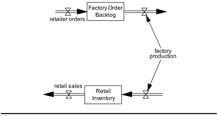
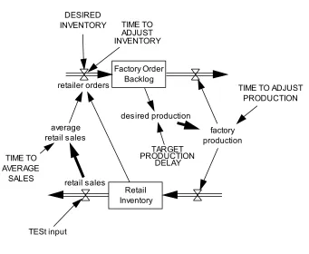
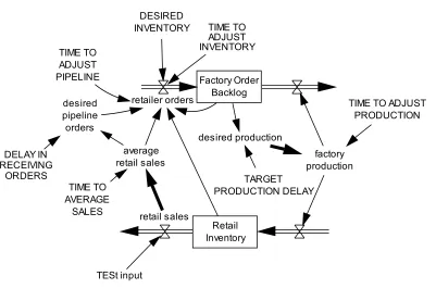
A basic stock and®ow diagram for the system we will consider is shown in Figure 5.11_{. There are two}_®_{ow processes: The production process shown at the} top of the±gure with a®ow to the right, and the distribution system shown at the bottom of the±gure with a®ow to the left. The production system is a®ow oforders, while the distribution system is a®ow ofmaterials. The two processes are tied together byfactory production, as shown at the right side of the±gure. As items are produced, the orders for these items are removed from the Factory Order Backlog, and the items are placed into Retail Inventory.

Note the use of the small \clouds" which are shown at the right and left ends of the production and distribution processes. These clouds represent either a source or a sink of ®ow which is outside the process that we are considering. For example, the cloud in the upper right corner of the±gure shows that we are not considering in our analysis what happens to orders once they have initiated factory production. (In an actual system, the orders probably continue to ®ow into a billing process. That is outside the bounds of what we are interested in

(2)

retailer orders

factory production

retail sales

Retail Inventory Factory Order

Backlog

Figure 5.1 A simple production-distribution system

here, and therefore we simply show a cloud into which the orders disappear|a \sink".)

The production-distribution system shown in Figure 5.1 is simpler than most real systems. These often involve multiple production stages, and also multi-ple distribution stages (for exammulti-ple, distributor, wholesaler, and retailer), each of which has an inventory of goods. Thus, it might seem that this example is too simple to teach us much that is interesting about real-world production-distribution processes. Surely our intuition will be su° cient to quickly ±nd a good way to run this system! Perhaps not. As we will see, this simpli±ed production-distribution system is still complicated enough to produce counter-intuitive behavior. Furthermore, this behavior is typical of what is seen in real production-distribution systems.

We will study the policy that the retailer uses to place orders with the fac-tory, and we will develop ±ve di erent models to investigate di erent policies for placing these orders. As we will see, it is not necessarily straightforward to develop an ordering policy that has desirable characteristics.

5.1 The First Model

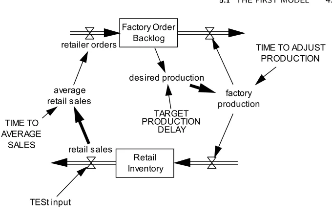
Figure 5.2, which has three parts, shows the ±rst model for the production-distribution system, and the four other models which follow will also be shown with analogous three-part±gures. Figure 5.2a shows the stock and®ow diagram for the±rst model, Figure 5.2b shows the Vensim equations for this model, and Figure 5.2c shows the performance of key variables within the process.

(3)

5.1 THE FIRST MODEL 45

average retail sales

retailer orders

TESt input

TIME TO ADJUST PRODUCTION

TARGET PRODUCTION

DELAY

factory production desired production

retail sales TIME TO

AVERAGE SALES

Backlog

Figure 5.2a Stock and ¯ow diagram for rst model

name starts with three capital letters, we know that it varies over time in a prespeci±ed manner. A variable which has a prespeci±ed variation over time is called anexogenous variable.

In the center of the Figure 5.2a diagram, an auxiliary variable \desired pro-duction" has been added, along with an auxiliary constant \TARGET PRO-DUCTION DELAY." Finally, at the right-center of the diagram, the auxiliary constant \TIME TO ADJUST PRODUCTION" has been added.

Factory Production

(4)

That is, the philosophy underlying this production system is that the retail or-derer should be able to predict the length of time it will take to receive an order that is placed. Thus, if the TARGET PRODUCTION DELAY is two weeks, the factory will attempt to set production so that the current Factory Order Backlog will be cleared in two weeks. In equation form, this says that

desired production = Factory Order Backlog TARGET PRODUCTION DELAY

where the Factory Order Backlog is measured in units of the item being produced, and the TARGET PRODUCTION DELAY is measured in weeks.

In typical realistic factory settings, production cannot be instantaneously changed in response to variations in orders because it takes time to change pro-duction resources, such as personnel and equipment. A more complex model of production would include explicit consideration of each of these factors, but we will approximate them here by saying that there is an average delay of TIME TO ADJUST PRODUCTION before the actual \factory production" is brought into line with \desired production."

In most realistic settings, the rate at which production can be adjusted varies depending on the immediate circumstances. Thus, the delay would not always be exactly equal to TIME TO ADJUST PRODUCTION. A simple model for this, but one which matches the data for many realistic settings, is that the time it takes to adjust production follows an exponential delay process. We will consider this particular approach in further detail below, but for now just consider the delay in bringing actual production into line with desired production to be variable with an average length of TIME TO ADJUST PRODUCTION.

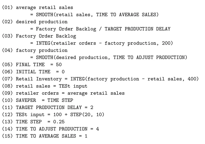
The equations for the production process, as well as the rest of the±rst model for the production-distribution system, are shown in Figure 5.2b. Equation 12 of this±gure shows that the TARGET PRODUCTION DELAY is 2 weeks, and equation 15 shows that the TIME TO ADJUST PRODUCTION is 4 weeks. (The values for these and other constants in the production-distribution model are illustrative and not intended to necessarily represent good management practice.) Equation 2 shows that the desired production is given by the equation dis-cussed earlier. Equation 4 shows that actual factory production is delayed from desired production by an average time of TIME TO ADJUST PRODUCTION. (In Vensim, the exponential delay function is called SMOOTH.)

When setting up a process model, it is important to keep the measurement units that you use consistent. If you use units of \weeks" of time in one place and \months" in another, then you will obviously get incorrect answers. (Note that you can set up a Vensim model to automatically check units. To simplify the presentation, we are not using this feature in our model.)

(5)

5.1 THE FIRST MODEL 47

(01) average retail sales

= SMOOTH(retail sales, TIME TO AVERAGE SALES) (02) desired production

= Factory Order Backlog / TARGET PRODUCTION DELAY (03) Factory Order Backlog

= INTEG(retailer orders - factory production, 200) (04) factory production

= SMOOTH(desired production, TIME TO ADJUST PRODUCTION) (05) FINAL TIME = 50

(06) INITIAL TIME = 0

(07) Retail Inventory = INTEG(factory production - retail sales, 400) (08) retail sales = TESt input

(09) retailer orders = average retail sales (10) SAVEPER = TIME STEP

(11) TARGET PRODUCTION DELAY = 2 (12) TESt input = 100 + STEP(20, 10) (13) TIME STEP = 0.25

(14) TIME TO ADJUST PRODUCTION = 4 (15) TIME TO AVERAGE SALES = 1

Figure 5.2b Vensim equations for rst model

Retailer Ordering

We now turn our attention to retail sales and orders to the factory by the re-tailer. We will assume that retail sales are predetermined. (That is, they are an exogenous variable to the portion of the process we are modeling.) We will soon consider what these orders are, but±rst we specify a procedure that the retailer uses to order from the factory.

The simplest ordering procedure is to order exactly what you sell. However, in practice, most retailers cannot instantly order each time they make a sale. Thus, ordering is based on an average over some time period. Furthermore, this average is likely to take into account recent trends. For example, if sales over the last few days have been up, then the retailer is likely to put more weight on that than on the lower sales of an earlier period.

A simple model of this type of averaging process is calledexponential smooth-ing, and this will be studied in more detail later. For now, you can consider that this type of averaging is approximately taking an average over a speci±ed period of time, but that more weight is given to recent sales than earlier sales. Thus, in the Figure 5.2a stock and ®ow diagram, the variable \average retail sales" is calculated by taking an exponential smooth of \retail sales" over the period TIME TO AVERAGE SALES. This is shown by equation 1 in the Figure 5.2b Vensim equations, and equation 15 shows that TIME TO AVERAGE SALES is equal to 1 week.

(6)

exponential averaging process and an exponential delay process are identical, and thus the same function is used for these in Vensim. However, conceptually the two processes are somewhat di erent. For the delay, we are interested in how long it takes for something in the future to happen. For the average, we are interested in what the average was for some variable over a past period.

The retailer ordering equations are completed by equation 9 in Figure 5.2b, which says that retailer orders are equal to average retail sales.

Test Input

To complete this ±rst model of the production-distribution system, we need to determine \retail sales." Equation 8 of Figure 5.2b shows that these are equal to \TESt input," and thus we need to specify this. Actual retail sales typically have some average value with random ®uctuation around this average. There may also be seasonal variation and an overall trend, hopefully upward. Thus, your±rst thought is probably to use a complex test input which represents these features of the real world.

However, we will use a very simple test input, and it is important to under-stand why this particular input is used because it is often used as a test input for process simulation models. The input we use will be a simple step: The input will start at one level, remain constant at that level for a period, and then jump instantly to another level and remain constant at the new level for the remainder of the period studied. The implementation of this input is shown in equation 12 of Figure 5.2b. The function STEP is de±ned by the following equation:

STEP(height;step time) = 0; Time<step time height; otherwise

That is, the function is zero until the time is equal to \step time," and then it is equal to \height." Thus, equation 12 of Figure 5.2b says that TESt input is equal to 100 units per week until the time is 10 weeks, and then TESt input is equal to 120 units per week for the remainder of the time.

Why is this used as a test input? It seems quite unlikely that the actual sales would have this form! The reason for using this form of test input has to do with what we are trying to accomplish with our model, and thus we need to discuss the purpose of our modeling.

Our primary purpose in constructing this model is to determine ways to im-prove the performance of the production-distribution process. In particular, we are studying di erent possible retailer ordering policies and how these impact the performance of the entire production-distribution process. There are, of course, many di erent possible patterns of retail sales, and we want to make sure that the particular pattern that we use in our model allows us to study the charac-teristics of the process that are important to understand if we are to improve the performance of the process. Remarkably, a step pattern for the retail sales is a good pattern for this purpose.

(7)

5.1 THE FIRST MODEL 49

retail orders and show that the behavior of the production-distribution process in response to this more realistic pattern is remarkably similar to its behavior with a step input. If you have studied engineering systems, you have probably already learned that the response of a linear system to a step input completely characterizes the behavior of the system. While the processes that we are consid-ering are generally nonlinear, their responses to a step input still gives important information about how the process responds to a variety of inputs.

To continue this theoretical discussion slightly longer, readers who have stud-ied Fourier or Laplace analysis methods will remember that the frequency spec-trum for a step function contains all frequencies. Therefore, using a step as input to a process excites all resonant frequencies of the process. These resonant frequencies are usually a critical determinant of the behavior of the process, and therefore the process response to a step input is often a good indicator of how the process will respond to a variety of inputs.

Other Model Equations

The remainder of the model equations in Figure 5.2b are mostly straightforward. Equations 3 and 7 for the stock variables Factory Order Backlog and Retail Inventory are known from the stock and ®ow diagram in Figure 5.2a, except for the initial values. We see from equation 3 that the initial value of Factory Order Backlog is 200 units, and equation 7 shows that the initial value of Retail Inventory is 400 units.

At an initial Factory Order Backlog of 200 units with a TARGET PRODUC-TION DELAY of 2 weeks (as given by equation 11 in Figure 5.2b), the \desired production" is 200=2 = 100 units per week. As long as there is no variation in Factory Order Backlog, then \factory production" will be equal to \desired production," and hence will also be equal to 100 units per week.

We see from equation 12 that the initial value of TESt input is 100 units per week, and hence from equation 8 this is also the initial value of retail sales. With no variation in retail sales, average retail sales will be equal to retail sales, and hence also equal to 100 units per week, and thus from equation 9 this will also be the retailer orders to the factory.

Since initial retail sales, and hence retailer order to the factory, are equal to factory production (100 units per week), then the system will initially be rather boring|the factory will make 100 units per week, which will be sold by the retailer. The Factory Order Backlog will remain stable at 200 units, and the Retail Inventory will remain stable at 400 units.

When a process is in a situation like that described in the last few paragraphs where the variables remain constant over time, it is said to be inequilibrium or steady state. A steady state condition for a simulation model can be detected by examining the stocks in the model. In steady state, the sum of all in®ows to each stock is equal to the sum of all out®ows, and therefore the magnitudes of the stocks do not change over time.

(8)

Backlog had been greater than 200 units, then this level would have declined over timeeven if retail sales had remained steady at 100 units per week. This is because at a Factory Order Backlog greater than 200 units factory production will exceed 100 units per week, which is the retailer order rate, and hence the

®ow out of Factory Order Backlog will exceed the®ow in.

Since our purpose in this analysis is to study the impact of changes in retail sales on the production-distribution process, it is desirable to start the process model in steady state. Otherwise, it will be di° cult to separate variations over time in the values of the various model variables which are due to changes in retail sales from those variations which are due to the lack of initial steady state. Similar arguments hold for many business process models, and it is usually good practice to initialize the variables in a model so that it starts in steady state.

The remaining equations in Figure 5.2b (equations 5, 6, 10, and 13) set char-acteristics of the simulation model. From equations 5 and 6 we see that the simulation will run for 50 weeks, or approximately one year. The rationale for setting the TIME STEP (equation 13) to 0.25 will discussed below.

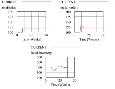
5.2 Performance of the Process

Before reviewing Figure 5.2c which shows results from simulating the model in Figure 5.5a and Figure 5.2b, you may wish to consider how you expect the process to respond to the TESt input. This is a much simpler production-distribution system than many in the real world, and many of those real world systems are managed with relatively little analysis. Perhaps all this analysis is not necessary. What do you think will happen in the process? Is the retailer ordering policy used in this model a good one? What are its strengths and weaknesses?

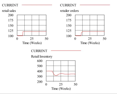
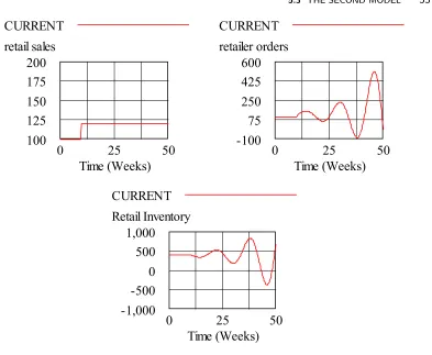
Figure 5.2c shows plots of three key variables (retail sales, retailer orders, and Retail Inventory) when the simulation model in Figure 5.2b is run. For the±rst ten weeks everything remains constant. The graphs show that retail sales are 100 units per week, and retailer orders also remain at 100 units per week. Retail Inventory remains at 400 units. At week 10, retail sales jump to 120 units per week, and remain there for the remaining 40 weeks shown in the graph. Retailer orders do not immediately jump to 120 units per week because an average of past sales is used as a basis for ordering, and it takes a while for the average to climb to 120 units. However, since the averaging period (TIME TO AVERAGE SALES) is only 1 week, retailer orders quickly move upward, and by week 14 these are also at 120 units per week.

A careful reader may wonder why these orders do not reach 120 units per week by week 11 since the TIME TO AVERAGE SALES is only 1 week. An exponential averaging process actually considers a period longer than the aver-aging time, but it gives increasingly less weight to earlier values as time goes on. This will be discussed further below.

(9)

5.2 PERFORMANCE OF THE PROCESS 51

CURRENT

retail sales

200

175

150

125

100

0

25

50

Time (Weeks)

CURRENT

retailer orders

200

175

150

125

100

0

25

50

Time (Weeks)

CURRENT

Retail Inventory

600

500

400

300

200

0

25

50

Time (Weeks)

Figure 5.2c Plots for rst model

to a peak of about 350 units at week 26 before dropping back to 340 units. Note that there is also a slight valley at around week 35.

This type of wiggling is calledoscillation. When you did your intuitive predic-tion of how the process would perform, did you expect this oscillapredic-tion? For that matter, did you predict that Retail Inventory would decline? While not shown in Figure 5.2c, after seeing this ±gure you will probably not be surprised to learn that Factory Order Backlog and factory production also both show similar oscillation to those shown by Retail Inventory.

While these oscillations are not large, they pose some challenges to a fac-tory manager. Decisions have to be made about how to provide the necessary resources under oscillating production conditions. For example, do you lay o factory workers when production dips? Also, the revenue stream associated with oscillating conditions is likely to be uneven, which is generally not desirable.

(10)

suppose that retail sales continue to grow (as we would hope they do!). What happens then? In that case, because average retail sales will always be somewhat less than current retail sales, there will never be quite enough ordered to replace what is sold, and eventually Retail Inventory will be depleted.

This e ect can be reduced by reducing the TIME TO AVERAGE SALES, which corresponds to more rapidly ordering, however, it cannot be entirely elim-inated because even if you instantaneously order after each sale, you will still fall behind because of delays in production.

This e ect is one reason that many production-distribution systems are mov-ing to automated, speeded-up ordermov-ing systems. For example, Wal Mart has made extensive use of such systems in its rise to retailing dominance. However, there is a limit to what is possible along these lines, particularly in businesses where the supply chain is not yet highly integrated. Is there some approach that a retailer can use in ordering that will reduce the danger of running out of inventory when sales rise? (Incidentally, note that if sales steadily fall, then Retail Inventory will steadily rise.)

5.3 The Second Model

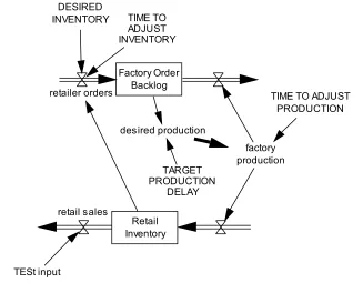
It seems that we need to directly consider the level of Retail Inventory when retailer orders are placed in order to make sure that this inventory does not reach undesirable levels. The stock and ®ow diagram in Figure 5.3a shows an approach to doing this. This is modi±ed from the Figure 5.2a diagram as follows: There is an information arrow from Retail Inventory to retailer orders to show that these orders depend on Retail Inventory. There are two auxiliary constants DESIRED INVENTORY and TIME TO ADJUST INVENTORY which also in®uence retailer orders. The remainder of this diagram is the same as Figure 5.2a.

The approach to considering Retail Inventory in retailer orders which is shown in this diagram makes intuitive sense: There is a speci±ed level of DESIRED INVENTORY and retailer orders are adjusted to attempt to maintain this level. Of course, we do not want to radically change our orders for every small change in Retail Inventory, and so we take some time to make the adjustment (TIME TO ADJUST INVENTORY). Turning this into a speci±c equation, there is now a component of retailer orders as follows:

DESIRED INVENTORY_£ Retail Inventory TIME TO ADJUST INVENTORY

(11)

5.3 THE SECOND MODEL 53

DESIRED

INVENTORY TIME TO ADJUST INVENTORY

retailer orders

TESt input

TARGET PRODUCTION

DELAY

AVERAGE SALES

Backlog

Figure 5.3a Stock and ¯ow diagram for second model

The equations for the second model are shown in Figure 5.3b. These are identical to the equations in Figure 5.2b except that de±nitions have been added for the two constants DESIRED INVENTORY and TIME TO ADJUST IN-VENTORY, and the equation for retailer orders has been modi±ed as discussed in the preceding paragraph. Speci±cally, in Figure 5.3b, equation 2 shows that the DESIRED INVENTORY is 400 units (which was the initial level of Retail Inventory), and equation 15 shows that the TIME TO ADJUST INVENTORY is 2 weeks. Equation 10 shows that retailer orders now include the component discussed above to adjust the level of Retailer Inventory, in addition to the com-ponent to replace retail sales.

(12)

(01) average retail sales = SMOOTH(retail sales, TIME TO AVERAGE SALES) (02) DESIRED INVENTORY = 400

(03) desired production = Factory Order Backlog / TARGET PRODUCTION DELAY (04) Factory Order Backlog

(07) INITIAL TIME = 0

(10) retailer orders = average retail sales

+ (DESIRED INVENTORY - Retail Inventory) / TIME TO ADJUST INVENTORY (11) SAVEPER = TIME STEP

(12) TARGET PRODUCTION DELAY = 2 (13) TESt input = 100 + STEP(20,10) (14) TIME STEP = 0.25

(15) TIME TO ADJUST INVENTORY = 2 (16) TIME TO ADJUST PRODUCTION = 4 (17) TIME TO AVERAGE SALES = 1

Figure 5.3b Vensim equations for second model

Thinking further along those lines, you will see that there is also no constraint in the model on the possible values for Factory Order Backlog and Retail Inven-tory. Thus, it is possible in this model for these to become negative. Again, a more complete model should take these issues into consideration. However, we are interested at the moment in the general characteristics of the performance of this process, rather than the details. The model we have developed will be su° cient for this purpose, as we will shortly see.

What do you think will be the performance of the modi±ed ordering policy? Do you think it will cure the problem of under ordering when sales are growing and over ordering when sales are declining?

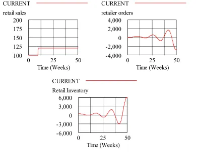
Figure 5.3c gives the answer, and it is not pleasant. The same three variables are plotted here as in Figure 5.2c which we considered earlier. We see that the system goes into large and growing oscillation. In fact, the situation is worse than it may ±rst appear because the scales for some of the graphs is Figure 5.3c (as shown on the left side of the graphs) are greater than those for Figure 5.2c. Thus, the oscillations are greater than it might ±rst appear by visually comparing Figure 5.2c and Figure 5.3c.

(13)

5.3 THE SECOND MODEL 55

CURRENT

retail sales

200

175

150

125

100

0

25

50

Time (Weeks)

CURRENT

retailer orders

600

425

250

75

-100

0

25

50

Time (Weeks)

CURRENT

Retail Inventory

1,000

500

0

-500

-1,000

0

25

50

Time (Weeks)

Figure 5.3c Plots for second model

behavior shown here. However, it is clear that the revised retailer ordering policy is highly unacceptable.

(14)

A Technical Note

Our main emphasis is on model formulation, but a brief note is in order on how the model equations are solved to develop a graph like the one shown in Figure 5.3c. As our earlier development showed, the solution of the model equations re-quires that some integrals be calculated. There are a variety of di erent methods to do this, and most simulation packages provide options for how this is done. The simplest of these methods, called Euler integration, was used to determine Figure 5.3c (as well as all the other output presented in this text).

The Euler integration method implemented in Vensim consists of the following steps:

1 Set \Time" to its initial value.

2 Set all of the stocks in the model to their initial values as speci±ed by the \initial value" argument of the INTEG function for each stock.

3 Compute the rate of change at the current value of \Time" for each stock by computing the net values of all the®ows®ow into and out of each stock. (That is,®ows into a stockincrease the value of the stock, while®ows out of a stock decrease the value of the stock.)

4 Assume that the rate of change for each stock will be constant for the time interval from \Time" to \Time + TIME STEP," and compute how much the stock will change over that interval. This can be expressed in equation form as follows: If the rate of change for a particular stock calculated in Step 3 is \rate(Time)," then the value of that stock at time Time + TIME STEP is given by

Stock(Time + TIME STEP) = Stock(Time) + TIME STEP¤rate(Time) 5 Add \TIME STEP" to \Time."

6 Repeat Steps 3 through 5 until \Time" reaches \FINAL TIME."

From this procedure, it is apparent that the accuracy of the Euler method is in®uenced by the value chosen for the model constant TIME STEP. It is generally recommended that a value of TIME STEP be selected that is less than one-third of the smallest time-related constant in the model. In the Figure 5.3b model, the smallest such constant is TIME TO AVERAGE SALES which is equal to 1 week. Therefore, TIME STEP was set equal to 0.25, which is one-quarter of TIME TO AVERAGE SALES. A quick test for whether TIME STEP is small enough is to reduce it by a factor of two and rerun the simulation. If there is no signi±cant change in the output, then this indicates that TIME STEP is small enough.

(15)

5.5 THE FOURTH MODEL 57

More sophisticated integrated methods available in many simulation packages often include one or more of the Runge-Kutta methods. The underlying idea of these methods is to estimate the rate at which the®ows into stocks are varying over time, and then use this information to improve on the approximation in Step 4 of the Euler procedure presented above. When this is done, it is often possible to achieve improved accuracy without as much increase in computation as would be necessary if the value of TIME STEP were decreased in the Euler procedure.

5.4 The Third Model

You might suspect that the problem displayed in Figure 5.3c is due to including a component in the retailer orders to take account of retail sales. Perhaps if we focus completely on Retail Inventory when making retailer orders, this will±x the problem. The stock and®ow diagram in Figure 5.4a shows this approach. This di ers from the diagram in Figure 5.3a in that the variables related to ordering to replace retail sales are removed. Speci±cally, at the left center of the diagram, the auxiliary variable \average retail sales" is removed along with the constant TIME TO AVERAGE SALES.

The corresponding equations are shown in Figure 5.4b. These di er from the equations in Figure 5.3b in that the equations for \average retail sales" and TIME TO AVERAGE SALES are removed, and the term for average retail sales is removed from equation 9 for retailer orders.

The resulting performance is shown in Figure 5.4c, and we see that this per-formance is even worse than what was shown in Figure 5.3c. (Note that the scales for some of the graphs in Figure 5.4c are considerably increased relative to Figure 5.3c, and thus the amplitude of the oscillations are much worse.)

Clearly this is not the answer.

5.5 The Fourth Model

Return now to the second model, whose performance is shown in Figure 5.3c. While the oscillations are clearly unacceptable, there is one way in which the performance of this process is better than the performance for the±rst model which was shown in Figure 5.2c. While there are wild oscillations in the Retail Inventory in Figure 5.3c, these oscillations are around an average level of 400 units, which is the Retail Inventory that we are trying to maintain. Thus, this process does not display the declining Retail Inventory level that is shown in Figure 5.2c. Unfortunately, the oscillations shown in Figure 5.3c are much too great to be acceptable in most real world production-distribution systems.

(16)

DESIRED

retailer orders

TESt input

TARGET PRODUCTION

DELAY

retail sales

Backlog

(17)

5.5 THE FOURTH MODEL 59

(01) DESIRED INVENTORY = 400 (02) desired production

= Factory Order Backlog / TARGET PRODUCTION DELAY (03) Factory Order Backlog

(06) INITIAL TIME = 0

(09) retailer orders

= (DESIRED INVENTORY - Retail Inventory) / TIME TO ADJUST INVENTORY

(10) SAVEPER = TIME STEP (11) TARGET PRODUCTION DELAY = 2 (12) TESt input = 100 + STEP(20, 10) (13) TIME STEP = 0.25

(14) TIME TO ADJUST INVENTORY = 2 (15) TIME TO ADJUST PRODUCTION = 4

(18)

CURRENT

retail sales

200

175

150

125

100

0

25

50

Time (Weeks)

CURRENT

retailer orders

4,000

2,000

0

-2,000

-4,000

0

25

50

Time (Weeks)

CURRENT

Retail Inventory

6,000

3,000

0

-3,000

-6,000

0

25

50

Time (Weeks)

(19)

5.5 THE FOURTH MODEL 61

DELAY IN RECEIVING

ORDERS

TIME TO ADJUST PIPELINE

desired pipeline orders

DESIRED

retailer orders

TESt input

TARGET PRODUCTION DELAY

AVERAGE SALES

Backlog

Figure 5.5a Stock and¯ow diagram for fourth model

pipeline, and then we basically forget about these orders and keep ordering. As discussed above, this leads to the oscillatory performance of the process.

The stock and®ow diagram in Figure 5.5a shows one way to account for the orders that are in the pipeline. This diagram is developed from the diagram in Figure 5.3a (not Figure 5.4a!) as follows: An information arrow is added from Factory Order Backlog to retailer orders. Thus, the retailer ordering policy will now explicitly take into account the backlog of orders. How this is done is indicated by the new auxiliary variable \desired pipeline orders" in the center of the left side of the diagram, and the two new constants DELAY IN RECEIVING ORDERS and TIME TO ADJUST PIPELINE.

The \desired pipeline orders" are the amount we want to have on order at any time, and this depends on \average retail orders" and the DELAY IN RE-CEIVING ORDERS. In particular, we need to have an amount in the supply pipeline equal to the product of \average retail orders" and DELAY IN RE-CEIVING ORDERS if we are to continue to receive enough to replenish our sales on average. That is,

desired pipeline orders = average retail sales

¤DELAY IN RECEIVING ORDERS:

(20)

change our orders in response to changes in desired pipeline orders. Hence there is a constant TIME TO ADJUST PIPELINE which plays a similar role to TIME TO ADJUST INVENTORY. Therefore, there should be a component in the retailer order equation to account for orders in the supply pipeline as follows:

desired pipeline orders£ Factory Order Backlog TIME TO ADJUST PIPELINE :

The required model equations are shown in Figure 5.5b. The value of DE-LAY IN RECEIVING ORDERS is set to agree with TARGET PRODUCTION DELAY. Since the factory has set up a TARGET PRODUCTION DELAY of 2 weeks (equation 14), DELAY IN RECEIVING ORDERS is also set to this value in equation 2. The TIME TO ADJUST PIPELINE is also set to 2 weeks in equation 18. Finally, the additional retailer ordering term discussed above is added to retailer orders in equation 12.

The resulting process performance is shown in Figure 5.5c. This is substan-tially improved relative to what is shown in any of the earlier ±gures. The magnitude of oscillation for Retail Inventory is not much greater than in the original process in Figure 5.2c, but now the Retail Inventory fairly quickly re-turns to the desired level of 400 units. (Note that the scales for Figure 5.2c and Figure 5.5c are the same.) Retailer orders now rise above retail sales, but they then quickly drop back to the level of retail sales without the wild oscillations that were displayed in the second and third models. (This type of behavior is called an overshoot.) This performance is pretty good, although there is still some oscillation in Retail Inventory.

5.6 The Fifth Model

After some study of the fourth model, you might consider a possible enhancement to reduce the amount of oscillation. In the fourth model, a constant value is used for the DELAY IN RECEIVING ORDERS. Perhaps adding a forecast for this delay would improve the performance of the process. Figure 5.6a shows a stock and ®ow diagram for a process which includes such a forecast. The constant DELAY IN RECEIVING ORDERS shown in Figure 5.5a has been replace by an auxiliary variable \delivery delay forecast by retailer," which is shown in the upper left corner of the diagram. This forecast depends on a constant TIME TO DETECT DELIVERY DELAY and another auxiliary variable \delivery delay estimate." The \delivery delay estimate" depends on Factory Order Backlog and \factory production."

(21)

5.6 THE FIFTH MODEL 63

(01) average retail sales = SMOOTH(retail sales,TIME TO AVERAGE SALES) (02) DELAY IN RECEIVING ORDERS = 2

(03) DESIRED INVENTORY = 400 (04) desired pipeline orders

= DELAY IN RECEIVING ORDERS * average retail sales

(05) desired production = Factory Order Backlog / TARGET PRODUCTION DELAY (06) Factory Order Backlog

(09) INITIAL TIME = 0

+ (DESIRED INVENTORY - Retail Inventory) / TIME TO ADJUST INVENTORY + (desired pipeline orders - Factory Order Backlog)

/ TIME TO ADJUST PIPELINE (13) SAVEPER = TIME STEP

(17) TIME TO ADJUST INVENTORY = 2 (18) TIME TO ADJUST PIPELINE = 2 (19) TIME TO ADJUST PRODUCTION = 4 (20) TIME TO AVERAGE SALES = 1

(22)

CURRENT

retail sales

200

175

150

125

100

0

25

50

Time (Weeks)

CURRENT

retailer orders

200

175

150

125

100

0

25

50

Time (Weeks)

CURRENT

Retail Inventory

600

500

400

300

200

0

25

50

Time (Weeks)

(23)

5.6 THE FIFTH MODEL 65

<factory production> delivery delay

estimate TIME TO DETECT

DELIVERY DELAY

delivery delay forecast by

retailer

TIME TO ADJUST PIPELINE

desired pipeline orders

DESIRED

INVENTORY TIME TO_ADJUST INVENTORY

retailer orders

TESt input

TARGET PRODUCTION

DELAY

AVERAGE SALES

Backlog

Figure 5.6a Stock and¯ow diagram for fth model

to read. In this case, it avoids the need to run an information arrow from the original version of \factory production" in the right center of the diagram all the way to the top center of the diagram where the \delivery delay estimate" variable is located.

The forecasting submodel is an attempt to model what an actual retailer might be able to do to forecast what is happening at its supplier. Such a retailer is likely to have some idea of what Factory Order Backlog and \factory production" are at any time. The product of these yields an estimate of delivery delay:

delivery delay estimate = Factory Order Backlog factory production

However, the retailer's estimates of Factory Order Backlog and factory pro-duction are likely to be somewhat out of date at any given time, and also

(24)

discussed earlier. Thus, the \delivery delay forecast by retailer" is modeled as an exponential average of the \delivery delay estimate" over an averaging period of TIME TO DETECT DELIVERY DELAY.

The equations for the ±fth model are shown in Figure 5.6b. Equation 2 gives \delivery delay estimate," and equation 3 gives \delivery delay forecast by retailer." The constant TIME TO DETECT DELIVERY DELAY is given in equation 22 as 2 weeks.

Alas, as Figure 5.6c shows, adding this forecast makes things somewhat worse than in the fourth model. The process now oscillates. The basic problem is that forecasts tend to predict that current trends will continue into the future. Thus, when retail sales jump at 10 weeks, the forecast leads to more extreme over ordering than in the fourth model. This overcorrection problem also occurs during the later attempt to reduce ordering, and the oscillating process continues. Forecasts sometimes do not help system performance, as this example shows.

5.7 Random Order Patterns

At this point, some readers may say, \Yah, but this model is too simple. The real world is more complex than this, and things average out. You don't really have to worry about all this stu in the real world." While this is a natural reaction, it is a little strange when you think about it: A more complicated process will perform better and be easier to manage? This doesn't seem very likely. And the data doesn't support that view. The oscillatory behavior of production-distribution systems, as well as many other social-technical systems (including the national and world economies) is well documented.

As a small con±rmation of the more general applicability of what we have seen in this chapter, Figure 5.7 shows the performance of the second model and the fourth model that we studied above in the presence of random retail orders. To produce these diagrams, equation 12 of the second model (shown in Figure 5.3b) and the equivalent equation 16 of the fourth model (shown in Figure 5.5b) were replaced by

TESt input = 100 + STEP(20;10) RANDOM UNIFORM(0;1;0):

The Vensim function RANDOM UNIFORM(m, x, s) produces random numbers that are uniformly distributed between m and x, with the argument s (called the seed) setting the speci±c stream of random numbers. Therefore, this modi±ed equation will produce a TESt input of 100 until week 10, and then it will produce a random TESt input that is distributed uniformly between 100 and 120.

(25)

5.7 RANDOM ORDER PATTERNS 67

(01) average retail sales = SMOOTH(retail sales, TIME TO AVERAGE SALES) (02) delivery delay estimate = Factory Order Backlog / factory production (03) delivery delay forecast by retailer

= SMOOTH(delivery delay estimate, TIME TO DETECT DELIVERY DELAY) (04) DESIRED INVENTORY = 400

(05) desired pipeline orders

= delivery delay forecast by retailer * average retail sales (06) desired production = Factory Order Backlog / TARGET PRODUCTION DELAY (07) Factory Order Backlog

= SMOOTH(desired production,TIME TO ADJUST PRODUCTION) (09) FINAL TIME = 50

(10) INITIAL TIME = 0

(11) Retail Inventory = INTEG(factory production - retail sales,400) (12) retail sales = TESt input

+ (DESIRED INVENTORY - Retail Inventory) / TIME TO ADJUST INVENTORY + (desired pipeline orders - Factory Order Backlog)

/ TIME TO ADJUST PIPELINE (14) SAVEPER = TIME STEP

(18) TIME TO ADJUST INVENTORY = 2 (19) TIME TO ADJUST PIPELINE = 2 (20) TIME TO ADJUST PRODUCTION = 4 (21) TIME TO AVERAGE SALES = 1

(22) TIME TO DETECT DELIVERY DELAY = 2

(26)

CURRENT

retail sales

200

175

150

125

100

0

25

50

Time (Weeks)

CURRENT

retailer orders

200

170

140

110

80

0

25

50

Time (Weeks)

CURRENT

Retail Inventory

600

500

400

300

200

0

25

50

Time (Weeks)

(27)

5.7 RANDOM ORDER PATTERNS 69

CURRENT

retail sales

200

175

150

125

100

0

25

50

Time (Weeks)

CURRENT

retailer orders

400

300

200

100

0

25

50

Time (Weeks)

CURRENT

Retail Inventory

800

600

400

200

0

25

50

Time (Weeks)

(28)

CURRENT

retail sales

200

175

150

125

100

0

25

50

Time (Weeks)

CURRENT

retailer orders

200

170

140

110

80

0

25

50

Time (Weeks)

CURRENT

Retail Inventory

600

500

400

300

200

0

25

50

Time (Weeks)

(29)

5.9 REFERENCE 71

5.8 Concluding Comments

Production-distribution processes, and similar structures in service businesses, are widespread throughout industry. Understanding these processes is useful for any business person. The di° culty of controlling these processes which was displayed in this example is shared by many real world processes. The result in many such processes is a massive control structure to ensure stability. Unfor-tunately, such structures often make the processes strongly resistant to change when the external environment changes. In the remainder of this text, we will investigate ways of looking at processes that can help you in the search for better performance.

5.9 Reference

(30)