The Precision of Unconditional Estimators of the Equity Premium

(1)

The Precision of Unconditional Estimators of the Equity Premium

Samih Antoine Azar1

1 _{Faculty of Business Administration & Economics, Haigazian University, Beirut, Lebanon}

Correspondence: Samih Antoine Azar, Professor, Faculty of Business Administration & Economics, Haigazian University, Mexique Street, Kantari, Beirut, Lebanon. Tel/fax: 961-134-9230. E-mail: [email protected]

Received: December 22, 2014 Accepted: January 13, 2015 Online Published: January 14, 2015 doi:10.5430/afr.v4n1p143 URL: http://dx.doi.org/10.5430/afr.v4n1p143

Abstract

This paper has the purpose of providing unconditional estimators of the equity premium. In plain words the estimators are obtained by the constants in regressions of the equity premium on a constant. More than one specification is tried and more than one type of standard errors is implemented. The specifications include ordinary least squares, EGARCH, robust least squares, quantile regressions, and Markov switching regressions with two regimes. The analysis is repeated by adding in categorical variables that correspond to outliers. Theoretically these estimators of the equity premium are unbiased and consistent. All models are subjected to serial correlation tests on the residuals. These tests support the absence of serial correlation. This is conducive to the conclusion that the models are well specified and that the estimators are not only unbiased and consistent but also efficient. The paper gives point estimates and 95% confidence intervals of the equity premium, develops hypothesis tests, and reports point estimates of the standard errors. The results may help in assessing the magnitude of the equity premium and the precision with which this premium is measured.

Keywords: Equity premium, Unconditional estimators, Robust standard errors, EGARCH, Ordinary least squares, Robust least squares, Quantile regressions, Markov switching regressions, Categorical outlier variables

1. Introduction

The size of the equity risk premium has been the subject of intense investigation. Based on this research it is inferred that the equity premium is surely much larger than the short term T-bill rate. What is lacking in the literature is the extent of precision in estimating the equity premium. Rare are the studies that provide a standard error for the estimated equity premium. Dimson et al. (2008) are an exception. Other academicians, like Fama and French (2002) and Goetzmann and Ibbotson (2006), report point estimates and standard deviations from which it is difficult to derive standard errors. This paper finds that these standard errors are relatively large. Thus the major purpose of this paper is to offer as many precision estimates as possible by varying the model that is specified, while keeping these models simple. Two unbiased estimators of the equity premium are the unconditional mean and the unconditional median. The latter estimator is a natural input in quantile regressions. The first unconditional estimator can be obtained easily from a regression of the premium on a constant, and the precision of estimation is the precision with which this constant is estimated. More than one variant of this basic model is attempted. There is more disparity than commonness in the results. Especially crucial is whether or not the standard errors need to be adjusted for serial correlation and heteroscedasticity. Robust standard errors tend to produce larger standard errors, and consequently less precision. In addition each variant specification provides for a point estimate of the equity premium that is generally different from other specifications. This paper intends to provide for the equity premium (1) point estimates with their respective t-statistics, (2) 95% confidence interval estimates, and (3) the appropriate standard errors. Of course a large standard error does not necessarily mean that precision is lost because some point estimates are larger than others. Surprisingly some interval confidence limits include negative realizations for the equity premium. This means that the hypothesis that the equity premium is in all cases and always positive may turn out to be untenable.

(2)

www.sciedu.ca/afr Accounting and Finance Research Vol. 4, No. 1; 2015

Published by Sciedu Press 144 ISSN 1927-5986 E-ISSN 1927-5994

because these regressions are effectively conditional on the selected dummy variables. However the fact that only dummy variables are included makes the models to approach closely an unconditional regression.

The paper is organized as follows. In the next section, section 2, some theoretical issues pertaining to the equity risk premium are covered. Section 3 is the empirical part where the regression results are presented and discussed. The last section is a conclusion.

2. Theory

The paradigm in the literature up until the late 1970s was that equities must earn higher returns than a safe asset, like a T-bill, as compensation for the additional systematic risk. The CAPM was at that time still the rule. Little interest was expressed on how large the equity premium is or should be. Concern about the size of the equity risk premium surfaced after the seminal paper by Mehra and Prescott (1985) was published. Mehra and Prescott showed that the equity premium is too large relative to theoretical expectations by building upon an appraised study by Lucas (1978). In fact they find that the coefficient of relative risk aversion needed to justify the equity premium must be as high as 50, which is unreasonable. A whole literature has emerged in order to explain this discrepancy or puzzle. The papers in the edited volume of Mehra (2008) are testimony to the richness of this literature. It is not the purpose of this paper to summarize the various theoretical efforts that have been made to reconcile theory with fact and to resolve the underlying puzzle. Let it be mentioned however that Weil (1989) transforms the puzzle of a too great actual equity premium to a puzzle of a too great theoretical risk-free rate.

Instead of trying to find out theoretical vindications for the puzzle some authors resorted to different agendas, like that of providing evidence that the expected, or normal, or theoretical, equity premium is less than the actual premium. See, for example, Arnott and Bernstein (2002), Fama and French, (2002), and Bostock (2004). However, by surveying the profession, Welch (2000) finds that financial economists estimate the just equity premium to be close to the actual one.

More recent research on estimating the equity premium has taken an accounting route. The basic model is the residual income model of Ohlson (1995), which relates the market value of equity to the sum of the book value of equity with the discounted future residual income. Easton et al. (2002) and Easton (2004) extend this basic Ohlson model to estimate simultaneously the cost of equity and the long term growth rate that occurs after the terminal date of the earnings forecast by financial analysts. This allows these authors to derive a simple linear regression equation in which the coefficients provide simultaneously estimates of the two target parameters, i.e. the cost of equity and the long run growth rate in earnings. The estimates of the cost of equity are averaged to obtain the aggregate equity premium. Nekrasov and Ogneva (2011) further refine the model of Easton et al. (2002) and Easton (2004) by showing that weighted least squares provide better individual and overall estimates. Fitzgerald et al. (2013) use similar equity valuation models and they simulate key variables. They take 3,012 alternative combinations of these variables and they plug these values into the valuation model. Fitzgerald et al. (2013) call their estimates unconstrained because “they are not constrained by the researchers’ growth rate assumption or by the assumption that all firms carrying the same industry label have identical cost of capital and growth estimates, and they are not constrained by the conversion of a discounted cash flow model to a linear form” (p.563). All these studies start by estimating the cost of equity for individual or for small portfolios and they aggregate these estimates to obtain the market equity premium. Unfortunately all the estimates remain still point estimates since the researchers fail to provide a measure of precision to their estimates. This paper has the essential purpose of filling this gap.

According to the Arbitrage Pricing Theory (APT), due to Ross (1976), the return on any financial asset is explained by a reaction to unexpected shocks, mostly macroeconomic in nature. If r~_it is the stochastic return on a financial asset i, and _itis an unexpected unsystematic or idiosyncratic shock with mean zero, E_t

 

_it 0 for each i, then the following is true through time t:

it jit j i

it r X

r   ~ 

~ _with

 

~ _₀

jit t X

E  j and i  E_t

 

r~_it E_t

 

r_i _i (1) The same applies to a return on a market index, and, additionally, to the market premium, which is the market return over the return on the risk-less asset. The thrust of this paper is to undertake variants of regressions on a constant, which represents r_i in equation (1). As demonstrated to the right-hand side of equation (1) this constant is an unbiased and consistent, but inefficient, estimator of the population mean return _i.The t-statistic on this constant is equivalent to a t-test on a measure of location with the following actual test statistic:

n s -c x tatistic

actual t-s  (2)

(3)

this constan an interval quantile reg quite adjac premium a formulae. T of -0.6614 These are d for both se implies tha estimates o larger. The are coupled 3. Empiric The data on of return in data is mon variable. T the T-bill r geometric independen half the va variance is premium b

There are t the second the sample constant. If an outlier. 1974, Nove In Table 1 regressions the regress by calculat

nt is overstated with more tha gressions this cent to each o are considered, The first series 12. The tests f distributed, un eries at low ma at the average of the equity pr e same issue ar d with large sta cal results

n the S&P 500 n the secondar nthly and span wo variable se rate is deducte rate is just the ntly and identi ariance of the s 4%, then one e smaller from

two general set is by includin e. These outlie f the realized re

The graph is e ember 1974, F

the empirical s, except for th sions in Table ting robust stan

d, because of o an 95% confide measure is the other. Otherwi , one calculate s of the equity for skewness p der the null hy arginal signific e lies to the le

remium are lar rises with Mar andard errors.

0 stock market ry market is re ns the period fr eries for the equ ed, and the geo e first differen cally distribute first. The stan e half of this v m the first by ar

ts of estimation ng in the regre

rs are identifie esidual falls ou exhibited just ebruary 1987, results of nine he EGARCH m

1 are as follow ndard errors ac

omitted variab ence. In most c e median. If the se the results ed from the ar

premium has a produce the fo ypothesis, as a cance levels. H eft of the med rger but this co rkov switching

index is obtain etrieved from t from early Mar uity premium a ometric return nce in the natu ed the average ndard deviation

ariance is 2%. round 2%. Unfo

n. The first set ssion, besides ed by inspectin utside the band

above. The se November 198 e variants of reg model, by inclu

ws. First regres cording to New

bles, (see equat cases the meas e distribution i may differ, a ithmetic perce a skewness of llowing two te standard norm Hence there is s

dian. In quanti omes at the ex g regressions w

ned from the w the web page o rch 1950 to ear are computed:

of the S&P 5 ural logs of th e of the second n of the equity . It is therefore fortunately the

t is by regressin the constant, 7 ng the recursiv d of plus or min ven outliers ar 87, September gressions on a uding in the est ssions on the c wey and West

tion (1), which sure of location is symmetric th and they actua entage change,

-0.428994, an est statistics re mal distribution strong evidence ile regressions pense of preci which provide r

web page of Ec of the Federal rly January 20 the arithmetic 00 from which he level series d estimate mus y returns is 20 e expected that empirical resu

ng the equity p 7 dummy varia ve residuals of nus two standa re on the early 1998, and Nov

constant are p timation the se constant with H

(1987). Then a

h makes a 95% n is the mean b he mean and th ally do. Two s

and the other nd the second s espectively -4.8 n. The null of s e for negative s, based on th sion as the sta relatively high

conStats. The d Reserve Bank 014, with 767 o

return on the S h the T-bill ra

of the S&P 5 st be lower tha 0% on average t the second m lts do not obey

premium plain ables represen f the least squ ard errors then y days ofDece vember 2008. presented. Tabl even dummies. HAC standard an EGARCH (N

% confidence in but in the case

he median sho series for the r from the geo series has a ske 85035 and -7.4 symmetry is re skewness. The he median, the andard errors ar h point estimat

data on the T-b k of Saint Loui observations o S&P 500 from ate is subtracte 500. If the seri an that of the f e, and as a res measure of the

y to this require

ly on a constan nting the 7 outl uares regression

it is considered ember 1973, O

le 2 repeats the The nine varia errors are con Nelson, 1991)

nterval e of the ould be equity ometric ewness 47815. ejected e latter e point re also es that bill rate is. The n each which d. The ies are first by ult the equity ement. nt, and liers in n on a d to be October

(4)

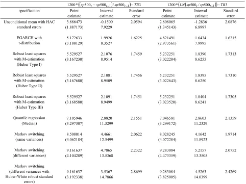
of the conditional variance is estimated with the additional assumption of a t-distribution. The mean equation includes only the constant. Then robust least squares are tried which adjust the regressions for outliers in the dependent variable, and these are estimated with three different types of robust standard errors (Huber, 1973, 1981). Then quantile regressions are implemented at the median of the series (Koenker and Basset, 1978; Basset and Koenker, 1982; Koenker, 1994; Koenker and Machado, 1999; and Koenker, 2005). And finally Markov switching regressions with two regimes are applied (Goldfeld and Quandt, 1973, 1976; Maddala, 1986; Hamilton, 1990, 1994; Frühwirth-Schnatter, 2006). One of the two regimes is selected. These switching regressions are carried out with the assumption of constant variances across regimes or with the assumption of different variances across regimes and finally with the use of robust standard errors together with regime-specific variances. All these specifications are repeated, except for the EGARCH model, with the inclusion of the 7 categorical variables that identify the 7 outliers in the data, making eight regressions in total instead of nine. In addition Tables 1 and 2 present regressions results with the two methods of the calculation of the return of the S&P 500 that is part of the equity premium, and which are by arithmetic returns and geometric returns.

Table 1. Plain regressions on the constant.

 

 500 500 / 500  3

*

1200 sp _tsp _t₁ sp _t₁ TB 1200*LNsp500t/sp500t1TB3

specification Point estimate

Interval estimate

Standard error

Point estimate

Interval estimate

Standard error Unconditional mean with HAC

standard errors

EGARCH with t-distribution

Robust least squares with M-estimation

(Huber Type I)

(Huber Type II)

(Huber Type III)

Quantile regression (Median)

Markov switching (same variances)

Markov switching (different variances)

Markov switching (different variances with Huber-White robust standard

errors)

3.886473 (1.887173)

5.172633 (3.188129)

5.529527 (3.167230)

5.529527 (3.167680)

5.529527 (3.168580)

7.105946 (3.297307)

8.508014 (4.062184)

9.161637 (4.104289)

9.161637 (3.192338)

-0.1500 7.9229

1.9926 8.3527

2.1076 8.9514

2.1081 8.9509

2.1091 8.9499

2.8820 11.3299

4.4661 12.5499

4.7865 13.5368

3.5367 14.7866

2.0594

1.6225

1.7459

1.7456

1.7451

2.1551

2.0622

2.2322

2.8699

2.808065 (1.345143)

4.821491 (2.973561)

5.232251 (3.022204)

5.232251 (3.022643)

5.232251 (3.023520)

7.046581 (3.299172)

8.028245 (4.072284)

9.283084 (4.473359)

9.283084 (3.825005)

-1.2836 6.8997

1.6434 7.9995

1.8390 8.6255

1.8395 8.6250

1.8404 8.6241

2.8603 11.2329

4.1642 11.8923

5.2157 13.3505

4.5263 14.0399

2.0876

1.6215

1.7313

1.7310

1.7305

2.1359

1.9714

2.0752

2.4269

Notes: In parentheses are t-statistics. sp500 stands for the S&P 500 stock market index. TB3 stands for the 3-month T-bill rate in the secondary market. LN is the natural logarithm. In the Markov switching regressions one of the two regimes is selected.

(5)

14.7866%, and the minimum of the upper limits of these intervals is 7.9229%. There is also some variation in the standard errors. The minimum standard error is 1.6225% and the maximum is 2.8699%.

In Table 1, and in what concerns the equity premiums obtained from geometric returns of the S&P 500, the point estimates range more widely than before between 2.808065% and 9.283084%. While the first estimate is lower by approximately 1% from its counterpart with arithmetic calculations, the second estimate is surprisingly higher than its arithmetic counterpart. This contradicts the expectation of a 2% lower point estimate for the statistics from geometric returns. Again whether these point estimates are plausible is an open question. All average equity premiums are statistically significantly different from zero, with the lowest t-statistic being 2.973561, except for the average obtained by HAC robust standard errors, (Newey and West, 1987), which carries a t-statistic of 1.345143. As a consequence the 95% confidence interval of the equity premium of this last regression includes negative realizations. For the remaining eight specifications the minimum limit of the 95% confidence intervals is an annualized 1.6434%, which is not that far from zero, while the maximum lower limit is 5.2157%. However the maximum of the upper limits of the same 95% confidence intervals is an annualized 14.0399%, while the minimum of the upper limits is 6.8997%. There is also some variation in the standard errors which are, however, always less than their counterparts with arithmetic calculation of the S&P 500 stock market returns. The minimum standard error is 1.6215% and the maximum is 2.4269%. This compares with a minimum standard error of 1.6225% and a maximum of 2.8699% with the arithmetic calculation.

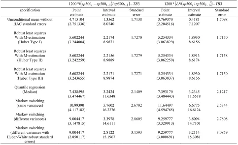
Table 2. Regressions on the constant including 7 dummy variables identified from the recursive residuals.

 

 500 500 / 500  3

*

1200 sp _tsp _t_₁ sp _t_₁ TB 1200*LNsp500_t/sp500_t_₁TB3 specification Point

estimate

Interval estimate

Standard error

Point estimate

Interval estimate

Standard error Unconditional mean without

HAC standard errors

Robust least squares With M-estimation (Huber Type I)

Robust least squares With M-estimation (Huber Type II)

Robust least squares With M-estimation (Huber Type III)

Quantile regression (Median)

Markov switching (same variances)

Markov switching (different variances)

Markov switching (different variances with Huber-White robust standard

errors)

4.715104 (2.751336)

5.602244 (3.244004)

5.602244 (3.242259)

5.602244 (3.243655)

7.438595 (3.474467)

10.99390 (4.117182)

9.004417 (3.147815)

9.004417 (2.850117)

1.3562 8.0740

2.2174 8.9871

2.2156 8.9889

2.2171 8.9874

3.2424 11.6348

5.7602 16.2276

3.3978 14.6111

2.8122 15.1967

1.7138

1.7270

1.7279

1.7271

2.1409

2.6702

2.8605

3.1593

3.769370 (2.204516)

5.254334 (3.063829)

5.254334 (3.062259)

5.254334 (3.063837)

7.393170 (3.484443)

11.64497 (4.594765)

9.259777 (3.329913)

9.259777 (3.000691)

0.4181 7.1207

1.8930 8.6156

1.8913 8.6174

1.8930 8.6156

3.2345 11.5518

6.6775 16.6124

3.8094 14.7101

3.2114 15.3081

1.7098

1.7150

1.7158

1.7150

2.1217

2.5344

2.7808

3.0859

Notes: See notes under Table 1. All regressions include 7 dummy variables. The dummies are respectively for the early days of December 1973, October 1974, November 1974, February 1987, November 1987, September 1998, and November 2008.

(6)

and the minimum of the upper limits of these intervals is 8.0740%. There is also some variation in the standard errors. The minimum standard error is 1.7138% and the maximum is 3.1593%.

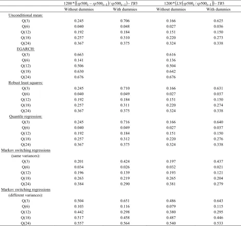
Table 3. Actual p-values of the Ljung-Box Q-statistics for the lag length specified in parentheses.

 

 500 500 / 500  3

*

1200 sp _tsp _t_₁ sp _t_₁ TB 1200*LNsp500_t/sp500_t_₁TB3

Without dummies With dummies Without dummies With dummies

Unconditional mean: Q(3) Q(6) Q(12) Q(18) Q(24) EGARCH:

Q(3) Q(6) Q(12) Q(18) Q(24) Robust least squares:

Q(3) Q(6) Q(12) Q(18) Q(24) Quantile regression:

Q(3) Q(6) Q(12) Q(18) Q(24)

Markov switching regressions (same variances):

Q(3) Q(6) Q(12) Q(18) Q(24)

Markov switching regressions (different variances):

Q(3) Q(6) Q(12) Q(18) Q(24)

0.245 0.040 0.192 0.257 0.367

0.663 0.141 0.506 0.630 0.676

0.245 0.040 0.192 0.257 0.367

0.201 0.034 0.196 0.263 0.384

0.504 0.103 0.442 0.517 0.557

0.706 0.048 0.184 0.310 0.375

0.710 0.049 0.184 0.311 0.375

0.716 0.049 0.184 0.312 0.375

0.424 0.026 0.139 0.219 0.290

0.651 0.116 0.298 0.458 0.564

0.166 0.027 0.151 0.220 0.324

0.616 0.136 0.504 0.642 0.676

0.166 0.027 0.151 0.220 0.324

0.197 0.032 0.193 0.265 0.381

0.486 0.079 0.380 0.487 0.540

0.625 0.036 0.150 0.273 0.338

0.631 0.037 0.150 0.274 0.338

0.640 0.037 0.150 0.276 0.338

0.437 0.021 0.121 0.204 0.279

0.643 0.115 0.295 0.446 0.533 Notes: See notes under Table 1 and Table 2. Robust standard errors do not affect the actual p-values of the Q-statistics. The actual p-values of the Q-statistics for the two EGARCH models are on the standardized residuals.

(7)

those in the previous paragraph. Again there is also some variation in the standard errors. The minimum standard error is 1.7098% and the maximum is 3.0859%.

An indicator of good specification is the absence of serial correlation in the residuals. Table 3 reports the actual p-values of the Ljung-Box Q-statistics for lag lengths of 3, 6, 12, 18, and 24 months. All Q-statistics are on the residuals except the Q-statistics on the EGARCH model which are on the standardized residuals. These are the residuals divided by the conditional standard deviations. The Q-statistics are not affected from estimation by robust standard errors. Hence there is no need to repeat the same p-values when robust standard errors are implemented. A vast majority of the p-values, close to unanimity, are above 5%, even above 10%, failing to reject the null of no serial correlation. However there is evidence that, when 6 months is chosen as the lag length, serial correlation becomes significant at the 5% marginal significance level but not at the 2% or 1% marginal significance levels. This should not come as a surprise, given the supremacy of the evidence for other lag lengths, and may be due to some kind of seasonality, or even just due to sampling error. Based on these Q-statistics all the models seem to be well specified. This implies that the X~js in equation (1) are non-existent or quite unstable for a market return, although they may

be important for specific individual financial assets, and this renders the estimators efficient in addition to being unbiased and consistent.

4. Conclusion

This paper provides for unconditional estimators of the equity premium, obtained by the constants in regressions of the equity premium on a constant. More than one specification and more than one type of standard errors are implemented. The specifications include ordinary least squares, EGARCH, robust least squares, quantile regressions, and Markov switching regressions with two regimes. The analysis is repeated by adding in categorical variables that represent the outliers that are beyond plus or minus two standard errors of the estimates of the recursive residuals. All models are subjected to serial correlation tests on the residuals. These tests support the absence of serial correlation. Consequently the models are well specified and the estimators are not only unbiased and consistent but are also efficient. The paper gives point estimates and 95% confidence intervals of the equity premium, develops hypothesis tests, and reports point estimates of the standard errors. The results help in evaluating the magnitude of the equity premium and the precision with which this premium is measured. Hereafter are statistics on the equity premiums. For the regressions with the arithmetic percentage rate of the S&P 500, the minimum of the lowest margins is -0.1500%, and the maximum of the lowest margins is 5.7602%. For these same regressions the minimum of the highest margins is 7.9229% and the maximum of the highest margins is 15.1967%. The point estimates are between 3.886473% and 10.99390%. For the regressions with the geometric formulae of the S&P 500, the minimum of the lowest margins is -1.2836%, and the maximum of the lowest margins is 6.6775%. For these same regressions the minimum of the highest margins is 6.8997% and the maximum of the highest margins is 16.6124%. The point estimates are between 2.808065% and 11.64497%. The lowest standard error is 1.6215% and the highest is 3.1593%. This compares with a standard error of 1.96% for the US in Dimson et al. (2008).

References

Arnott, R. D. & Bernstein, P. L. (2002). What risk premium is "normal"? Financial Analysts Journal, 58, 2, 64-85. http://dx.doi.org/10.2469/faj.v58.n2.2524

Basset, G. Jr., & Koenker, R. (1982). An empirical quantile function for linear models with i.i.d. errors. Journal of the American Statistical Association, 77, 378, 407-415. http://dx.doi.org/10.2307/2287261

Bollerslev, T., & Wooldridge, J. M. (1992). Quasi-maximum likelihood estimation and inference in dynamic models

with time varying covariances. Econometric Reviews, 11, 143-172.

http://dx.doi.org/10.1080/07474939208800229

Bostock, P. (2004). The equity premium. The Journal of Portfolio Management, 30, 2, 104-111. http://dx.doi.org/10.3905/jpm.2004.319936

Dimson, E., Marsh, P. & Staunton, M. (2008). The worldwide equity premium: a smaller puzzle. In Handbook of the equity risk premium, Mehra, R. (ed.), 467-504. http://dx.doi.org/10.1016/B978-044450899-7.50023-3

Easton, P. (2004). PE ratios, PEG ratios, and estimating the implied expected rate of return on equity capital.

Accounting Review, 79, 73–95. http://dx.doi.org/10.2308/accr.2004.79.1.73

(8)

Fama, E., & French, K. (2002). The equity premium. Journal of Finance, 57, 2, 637-659. http://dx.doi.org/10.1111/1540-6261.00437

Fitzgerald, T., Gray, S., Hall, J., & Jeyaraj, R. (2013). Unconstrained estimates of the equity risk premium. Review of Accounting Studies, 18:560–639. http://dx.doi.org/10.1007/s11142-013-9225-z

Frühwirth-Schnatter, S. (2006). Finite mixture and Markov switching models. New York: Springer Science + Business Media LLC.

Goetzmann, W. N., & Ibbotson, R. G. (2006). The equity risk premium, essays and explorations. New York: Oxford University Press.

Goldfeld, S. M., & Quandt, R. E. (`1973). A Markov model for switching regressions. Journal of Econometrics, 3-16. http://dx.doi.org/10.1016/0304-4076(73)90002-X

Goldfeld, S. M., & Quandt, R. E. (1976). Studies in nonlinear estimation. Cambridge, MA: Ballinger.

Hamilton, J. D. (1990). Analysis of time series subject to changes in regime. Journal of Econometrics, 45, 39-70. http://dx.doi.org/10.1016/0304-4076(90)90093-9

Hamilton, J. D. (1994). Time series analysis. Princeton: Princeton University Press.

Huber, P. J. (1973). Robust regression: asymptotics, conjectures and Monte Carlo. The Annals of Statistics, 1, 5, 799-821. http://dx.doi.org/10.1214/aos/1176342503

Huber, P. J. (1981). Robust statistics. New York: John Wiley & Sons. http://dx.doi.org/10.1002/0471725250

Koenker, R. (1994). Confidence intervals for regression quantiles. In Asymptotic statistics, Mandl, P. & Huskova, H. (eds) New York: Springer-Verlag, 349-359. http://dx.doi.org/10.1007/978-3-642-57984-4_29

Koenker, R. (2005). Quantile regression. New York: Cambridge University Press. http://dx.doi.org/10.1017/CBO9780511754098

Koenker, R., & Basset, G. Jr. (1978). Regression quantiles. Econometrica, 46, 1, 33-50. http://dx.doi.org/10.2307/1913643

Koenker, R. & Machado, J. A. F. (1999). Goodness of fit and related inference processes for quantile regression.

Journal of the American Statistical Association, 94, 448, 1296-1310. http://dx.doi.org/10.1080/01621459.1999.10473882

Lucas, R. E. Jr. (1978). Asset prices in an exchange economy. Economterica, 46, 1429-1445. http://dx.doi.org/10.2307/1913837

Maddala, G. S. (1986). Disequilibrium, self-selection, and switching models. In Handbook of econometrics, Griliches, Z. & Intriligator, M. D. (eds), Volume 3, Amsterdam: North-Holland.

Mehra, R. (ed) (2008). Handbook of the equity risk premium. Amsterdam: Elsevier. http://dx.doi.org/10.1016/B978-044450899-7.50006-3, http://dx.doi.org/10.1016/B978-044450899-7.50004-X Mehra, R., & Prescott, E. C. (1985). The equity premium: a puzzle. Journal of Monetary Economics, 15, 145-161.

http://dx.doi.org/10.1016/0304-3932(85)90061-3

Nekrasov, A., & Ogneva, M. (2011). Using earnings forecasts to simultaneously estimate firm-specific cost of equity and long-term growth. Review of Accounting Studies, 16, 414–457. http://dx.doi.org/10.1007/s11142-011-9159-2 Nelson, D. B. (1991). Conditional heteroskedasticity in asset pricing: a new approach. Econometrica, 59, 347–370.

http://dx.doi.org/10.2307/2938260

Newey, W. K., & West, K. D. (1987). A Simple, positive semi-definite, heteroskedasticity and autocorrelation-consistent covariance matrix. Econometrica, 55, 703–708. http://dx.doi.org/10.2307/1913610 Ohlson, J. A. (1995). Earnings, book values and dividends in equity valuation. Contemporary Accounting Research, 11,

661–687. http://dx.doi.org/10.1111/j.1911-3846.1995.tb00461.x

Ross, S. (1976). The arbitrage theory of capital asset pricing. Journal of Economic Theory, 13, 341–360. http://dx.doi.org/10.1016/0022-0531(76)90046-6

Weil, P. (1989). The equity premium puzzle and the risk-free rate puzzle. Journal of Monetary Economics, 24, 401-421. http://dx.doi.org/10.1016/0304-3932(89)90028-7