M E T H O D O L O G Y
Open Access
Transposon insertion profiling by
sequencing (TIPseq) for mapping LINE-1
insertions in the human genome
Jared P. Steranka
1,2, Zuojian Tang
3,4, Mark Grivainis
3,4, Cheng Ran Lisa Huang
2, Lindsay M. Payer
1,
Fernanda O. R. Rego
5, Thiago Luiz Araujo Miller
5,6, Pedro A. F. Galante
5, Sitharam Ramaswami
7, Adriana Heguy
7,
David Fenyö
3,4, Jef D. Boeke
4*and Kathleen H. Burns
1,2*Abstract
Background:Transposable elements make up a significant portion of the human genome. Accurately locating these mobile DNAs is vital to understand their role as a source of structural variation and somatic mutation. To this end, laboratories have developed strategies to selectively amplify or otherwise enrich transposable element insertion sites in genomic DNA.
Results: Here we describe a technique, Transposon Insertion Profiling by sequencing (TIPseq), to map Long INterspersed Element 1 (LINE-1, L1) retrotransposon insertions in the human genome. This method uses vectorette PCR to amplify species-specific L1 (L1PA1) insertion sites followed by paired-end Illumina sequencing. In addition to providing a step-by-step molecular biology protocol, we offer users a guide to our pipeline for data analysis, TIPseqHunter. Our recent studies in pancreatic and ovarian cancer demonstrate the ability of TIPseq to identify invariant (fixed), polymorphic (inherited variants), as well as somatically-acquired L1 insertions that distinguish cancer genomes from a patient’s constitutional make-up.
Conclusions: TIPseq provides an approach for amplifying evolutionarily young, active transposable element insertion sites from genomic DNA. Our rationale and variations on this protocol may be useful to those mapping L1 and other mobile elements in complex genomes.
Keywords:LINE-1, Targeted PCR, Next generation sequencing
Background
Long INterspersed Element-1 (LINE-1, L1) is one of the most abundant mobile DNAs in humans. With roughly 500,000 copies, LINE-1 sequences comprise about 17% of our DNA [1]. Although most of these exist in an in-variant (fixed) state and are no longer active, about 500 insertions of the Homo sapiens specific L1 sequences (L1Hs) are more variable and derive from a few ‘hot’ L1Hs that remain transcriptionally and transpositionally active [2–7]. The activity of LINE-1 results in transpos-able element insertions that are a significant source of
structural variation in our genomes [8–11]. They are re-sponsible for new germline L1 insertion events as well as the retrotransposition of other mobile DNA sequences in-cludingAluShort INterspersed Elements (SINEs) [12–15] and SVA (SINE/VNTR/Alu) retrotransposons [16]. Add-itionally, LINE-1 can propagate in somatic tissues, and somatically-acquired insertions are frequently found in human cancers [17–23].
Characterizations of transposable element sequences remain incomplete in part because their highly repeti-tive nature poses technical challenges. Using these high copy number repeats as probes or primer sequences can create signals or products in hybridization-based assays and PCR amplifications that do not correspond to discrete gen-omic loci. Moreover, both the absence of many common insertion variants from the reference genome assembly * Correspondence:[email protected];[email protected]
4
Institute for Systems Genetics, NYU Langone Health, New York, NY 10016, USA
1Department of Pathology, Johns Hopkins University School of Medicine, Baltimore, MD 21205, USA
Full list of author information is available at the end of the article
as well as the presence of hundreds of thousands of similar sequences together complicate sequencing read mappability. Detecting insertions that occur as low fre-quency alleles in a mixed sample presents an additional challenge, such as occurs with somatically-acquired in-sertions. Nevertheless, several recent studies describe strategies for mapping these elements and highlight LINE-1 continued activity in humans today. These methods include hybridization-based enrichment [24–29]; select-ive PCR amplification [6, 17, 30–39]; and tailored ana-lyses of whole genome sequencing reads [10,11, 18,19, 40,41].
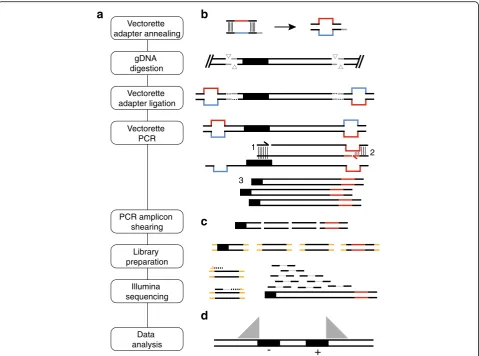
Here we present a detailed protocol to amplify and sequence human LINE-1 retrotransposon insertion loci developed in the Burns and Boeke laboratories, Trans-poson Insertion Profiling by sequencing (TIPseq) [22, 23,42–44]. This method uses ligation-mediated, vector-ette PCR [45] to selectively amplify regions of genomic DNA directly 3′of L1Hs elements. This is followed by library preparation and Illumina deep sequencing (see Fig.1a). TIPseq locates fixed, polymorphic, and somatic L1Hs insertions with base pair precision and deter-mines orientation of the insertion (i.e., if it is on the plus (+) or minus (−) strand with respect to the refer-ence genome). It detects, though does not distinguish between, both full length and 5′truncated insertions as short as 150 bp. TIPseq is highly accurate in identifying somatic L1 insertions in tumor versus matched normal tissues, and allows sequencing coverage to be efficiently targeted to LINE-1 insertion sites so it is an economical way to process samples for this purpose. We have used TIPseq to demonstrate LINE-1 retrotransposition in pancreatic [22] and ovarian [23] cancers, and to show that somatically-acquired insertions are not common in glioblastomas [44]. Together with the machine learning-based computational pipeline developed in the FenyӧLab for processing TIPseq data, TIPseqHunter [23], this protocol allows researchers to map LINE-1 insertion sites in human genomic DNA samples and compare insertion sites across samples.
Results
Experimental design
Starting material and optimal reaction size
High molecular weight genomic DNA is the starting material for TIPseq. This can be isolated from fresh or frozen tissues or cells. We typically use gDNA from phenol:chloroform extractions and ethanol precipita-tions, or from silica column preparations. This proto-col uses reaction sizes producing consistent results in our hands with starting material of 10μg genomic DNA (gDNA). We have successfully used a 3.3μg gDNA input ‘scaled-down’ protocol with comparable results to the full-scale protocol. However, we caution that smaller
reaction volumes will magnify effects of sample evap-oration or slight inaccuracies in pipetting. It is import-ant to maintain accurate reaction volumes at each step of the protocol. See Additional file 1: Table S1 for scaled-down reactions that start with as low as 3.3μg of gDNA.
Restriction enzyme selection
TIPseq uses 6 different restriction enzyme digests run in parallel to maximize the portion of the genome that is cut to a PCR-amplifiable fragment in at least one of the reactions. The combination of enzymes was selected using a greedy algorithm to maximize genomic frag-ments 1–5 kb long. An L1Hs insertion occurring at any location in the genome is highly likely then to be repre-sented by a fragment 1-3 kb in size in at least one of these parallel digests. This size balances informative-ness and amplification efficiency; longer fragments in-clude more sequence, but shorter fragments amplify more efficiently. For vectorette PCR to be successful, restriction enzymes should: 1) have a recognition cut site that occurs at the right genomic frequency (many 5- or 6- base pair cutters work well); 2) cut efficiently and independent of CpG methylation, 3) leave “stick-y-end”overhangs for ligation of the vectorette adapters, and 4) be able to be heat inactivated. Most importantly, no restriction enzyme should cut in the retroelement insertion at any position 3′ of the forward primer se-quence. This would prevent PCR amplicons from ex-tending into unique gDNA downstream of the element.
Vectorette adapter design
Pairs of vectorette oligonucleotides are annealed together to form double stranded vectorette adapters (see Table1). At one end of the vectorette, the two strands form compatible “sticky-ends” to the restriction enzyme di-gestion cut sites which allows for efficient adapter ligation (see Additional file2: Table S2). The vectorette central sequence is partially mismatched such that the vectorette primer sequence is incorporated on the bot-tom strand, but its reverse complement is missing from the top strand. This forces first stranded synthesis to occur out of the transposable element to create the vector-ette primer binding sequence. After this initial extension, exponential amplification can proceed in subsequent PCR cycles (see Fig.1b).
Specific primer selection
L1PA1 [also known as L1(Ta)] subset ofHomo sapiens -spe-cific LINE-1 (L1Hs). This strongly favors amplification of polymorphic and newly acquired somatic insertions and minimizes enrichment of older, “fixed present” elements.
Vectorette PCR conditions
Amplicons initiated within L1Hs insertions must traverse the LINE-1 polyA sequence and extend for a
significant distance into downstream gDNA. We use a touchdown PCR program to ensure a balance between promoting primer specificity and achieving high-yields. This program progressively lowers the an-nealing temperature of each cycle from 72 °C to 60 °C (see Table2). These cycling conditions, combined with the robust, proofreading DNA polymerase (ExTaq HS, Takara Bio; Shiga Japan), produces the complex mix-ture of optimally sized amplicons.
gDNA digestion
Vectorette adapter ligation
Vectorette adapter annealing
Vectorette PCR
PCR amplicon shearing
Library preparation
Illumina sequencing
Data analysis
1
2
3
+
-a
b
c
d
DNA shearing
We use a Covaris focused ultrasonicator (Covaris; Wo-burn, MA) with the manufacturer’s recommended set-tings to shear the vectorette PCR amplicons to 300 bp prior to library preparation (see Additional file 3: Fig-ure S2B). Shearing PCR amplicons may produce a broader size range than when shearing genomic DNA. If necessary, the treatment time may be modified on a per sample basis to adjust the final size distribution.
Library preparation and size-selection
Library construction may be performed using any kit that is compatible with Illumina next generation se-quencing, including Illumina’s TruSeq LT or PCR-free DNA sample prep kits (Illumina; San Diego, CA). We recommend using Kapa Library Preparation Kit for Illumina (Kapa Biosystems; Wilmington, MA) and to follow the manufacturer’s instructions. If necessary, amplification may be performed during library con-struction, however, we advise using a PCR-free library preparation. Library adapters add approximately 120 bp of length to the sheared DNA. It may be neces-sary to perform a size selection during library prepar-ation so that final library size is greater than 400 bp. This will prevent the generation of overlapping read pairs and reads containing adapter sequence. If ne-cessary, we recommend performing dual-SPRI bead selection during library preparation or adding Pippin prep selection (Sage Science; Beverly, MA) after li-brary pooling to remove all fragments smaller than 400 bp.
Illumina sequencing
Our data analysis pipeline, TIPseqHunter, requires 150 bp or shorter paired-end reads for optimal results. Longer
reads may be trimmed to meet this requirement. We rec-ommend a minimum of 15–25 million read pairs per sample. For example, for the Illumina HiSeq4000 this corresponds to pooling 12 samples per lane in high-output mode. These guidelines should result in suffi-cient coverage and read depth for identifying L1 inser-tion loci.
Data analysis
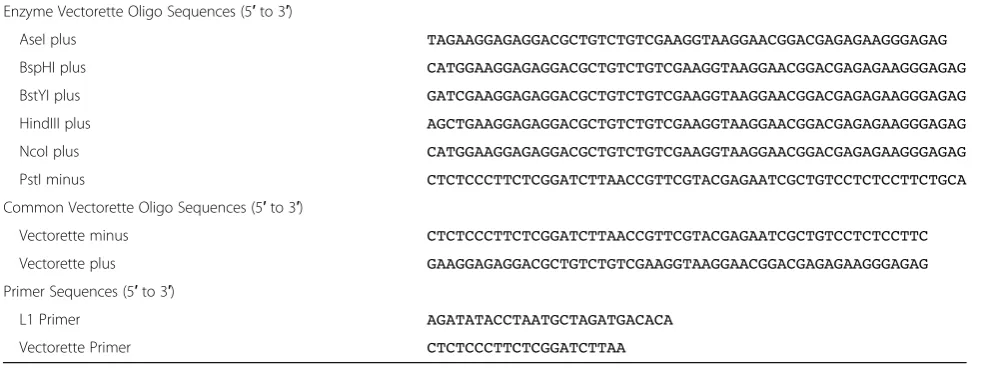
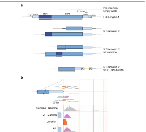
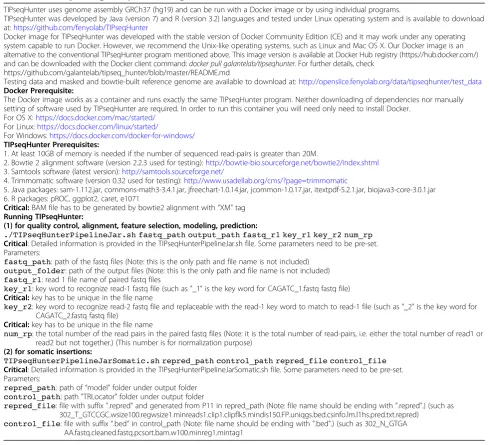
TIPseq produces reads that contain LINE-1 sequence, adjacent genomic sequence, or both (junction reads) (see Fig. 2b). TIPseq data analysis reveals precise, base-pair resolution of L1Hs insertions and their orientation). We recommend using our custom bioinformatics program: TIPseqHunter [23]. We developed this program with a machine learning algorithm that uses known insertions as a training set for identifying new insertions. TIPseq-Hunter is available for download at:https://github.com/ fenyolab/TIPseqHunter (see Table6). It is also available as a Docker image at: https://github.com/galantelab/tip-seq_hunter. This encapsulates all java dependencies, read aligners, genome indexes and biological annotation files needed by both steps of the pipeline. The genome in-dexes and annotation files in both TIPseqHunter and the Docker image use the human reference genome as-sembly GRCh37 (hg19). Instructions for use and down-load can be found in the README file at:https://github. com/galantelab/tipseq_hunter/blob/master/README.md. For sequencing runs of less than 20 million read pairs, 10–20 GB of RAM is suggested, and running time using 8 core processors on a Linux system is approximately 25 h. For runs in excess of 60 million reads, TIPseq-Hunter requires 40–50 GB of RAM, and running time is 1–1.5 h per 1 million reads. TranspoScope, a bioinformat-ics tool for browsing the evidence for transposable element Table 1Vectorette oligo and primer sequences
Enzyme Vectorette Oligo Sequences (5′to 3′)
AseI plus TAGAAGGAGAGGACGCTGTCTGTCGAAGGTAAGGAACGGACGAGAGAAGGGAGAG
BspHI plus CATGGAAGGAGAGGACGCTGTCTGTCGAAGGTAAGGAACGGACGAGAGAAGGGAGAG
BstYI plus GATCGAAGGAGAGGACGCTGTCTGTCGAAGGTAAGGAACGGACGAGAGAAGGGAGAG
HindIII plus AGCTGAAGGAGAGGACGCTGTCTGTCGAAGGTAAGGAACGGACGAGAGAAGGGAGAG
NcoI plus CATGGAAGGAGAGGACGCTGTCTGTCGAAGGTAAGGAACGGACGAGAGAAGGGAGAG
PstI minus CTCTCCCTTCTCGGATCTTAACCGTTCGTACGAGAATCGCTGTCCTCTCCTTCTGCA
Common Vectorette Oligo Sequences (5′to 3′)
Vectorette minus CTCTCCCTTCTCGGATCTTAACCGTTCGTACGAGAATCGCTGTCCTCTCCTTC
Vectorette plus GAAGGAGAGGACGCTGTCTGTCGAAGGTAAGGAACGGACGAGAGAAGGGAGAG
Primer Sequences (5′to 3′)
L1 Primer AGATATACCTAATGCTAGATGACACA
insertions into the genome by visualizing sequencing read coverage in regions flanking de novo insertion of transposable elements which are not present in the reference genome. TranspoScope can be downloaded at https://github.com/FenyoLab/transposcope and an in-structional video is available at:
https://www.youtube.-com/watch?v=exVAnoMRLSM.
Discussion
De novo insertion validation
TIPseqHunter accurately detects fixed, polymorphic, and de novo L1Hs insertions. Our previous studies have pro-duced validation rates has high as 96% [23]. While users can therefore be confident in TIPseqHunter calls, we recommend validating at least subsets of predicted
a
b
Full Length L1 Pre-insertion/ Empty Allele ORF2
5’UTR ORF1 3’UTR
TSD TSD
L1 primer
5’ Truncated L1
5’ Truncated L1 w/ Inversion
5’ Truncated L1 w/ 3’ Transduction
100 bp
Genome - Genome
L1 - Genome
Junction
All
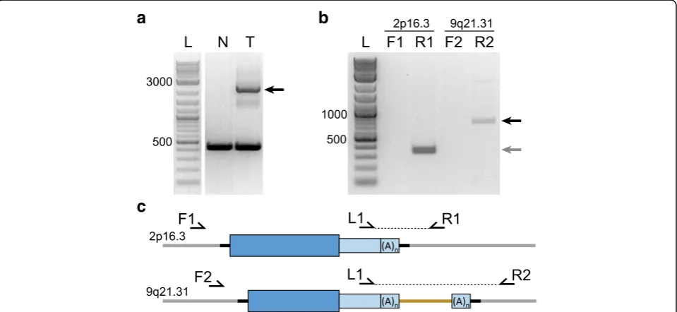
insertions whenever important conclusions are being drawn from a study. This can be accomplished by site-specific, spanning PCR and Sanger sequencing (see Table7). This will confirm the presence of the insertion and report the length and structure of the element. It is important to use the same high quality gDNA used in the TIPseq procedure to validation insertion candidates. Normal control DNA should be tested in parallel when validating somatic insertions from tumor-normal studies (see Fig. 3a). L1-specific 3’ PCR may be used to validate large insertions that are difficult to span in PCR and to identify possible 3′transduction events (see Table8).
Level of expertise required
The first part of the TIPseq protocol and final valida-tions (steps 1–21,31) require basic molecular biology equipment and techniques (digestion, ligation, and PCR). The second part of the protocol (steps 22–29) involves the use of more advanced equipment and methods (DNA shearing, library preparation, and deep sequencing). It is possible to contract ‘advanced’steps to sequencing core facilities depending on each user’s level of expertise and access to the required equip-ment, and this is our recommendation for users Table 2Vectorette PCR thermal cycler program
95 °C 5 min
95 °C 1 min 5 cycles
72 °C 1 min
72 °C 5 min
95 °C 1 min 5 cycles
68 °C 1 min
72 °C 5 min
95 °C 45 s 15 cycles
64 °C 1 min
72 °C 5 min
95 °C 45 s 15 cycles
60 °C 1 min
72 °C 5 min
72 °C 15 min
16 °C Hold
a
c
b
without training or experience with library preparation and deep sequencing. Data analysis (step 30) using TIPseqHunter and visualization using TranspoScope requires basic knowledge of NGS related bioinformat-ics and UNIX shell scripting experience in order to run the program from command line.
Applications of the method
TIPseq was initially adapted from a microarray based ap-proach called Transposon insertion profiling by micro-array or TIPchip [9, 42], which was first developed for mapping Ty1 elements inSaccharomyces cerevisae[42] . Although TIPseq is applicable to other transposable ele-ments or species, this protocol is optimized to detect LINE-1 insertions in the human genome, and currently our TIPseqHunter program can only process human LINE-1 TIPseq data. TIPseq may be used for a variety of applications, including: population studies to identify common structural variants, tumor vs. normal compari-sons to identify somatically-acquired insertions and trace cellular phylogenies, and in patients with specific pheno-types to evaluate for de novo retrotransposition events. Whole genome sequencing (WGS) can also be used for these purposes, and the main advantage of TIPseq is that insertion sites can be relatively deeply sequenced inex-pensively. Targeting sequencing to retrotransposon in-sertion sites can result in a 400x cost saving for L1Hs mapping, and a 60x cost savings forAlumapping.
Limitations of the method
Although TIPseq is a highly useful tool for detecting LINE-1 insertions, there are some limitations to the method that should be considered. First, TIPseq relies on restriction enzyme digestion of a large amount of high quality (high molecular weight) genomic DNA. For samples with limited amounts or reduced quality DNA, such as single-cell or fixed tissue, this protocol may need adjusted to work with similar efficiency. Sec-ondly, while this method provides insertion location and orientation information, it does not differentiate between insertion ‘types’. This includes classifying full length versus truncated insertions and elements with 5′ inversions or 3′transductions (see Fig.2a). While TIP-seq will detect these insertions, further analysis, such as gel electrophoresis or Sanger sequencing, is required to confirm insert size and sequence variations. Finally, TIPseq does not distinguish between heterozygous and homozygous insertion alleles. An additional qualitative validation, such as PCR, is needed to confirm zygosity.
Anticipated results
The TIPseq procedure should yield more than 10μg of purified PCR amplicons depending on vectorette PCR efficiency. The size distribution of these amplicons usually
averages 1-3 kb (see Additional file4: Figure S1A). This size distribution may vary depending on the quality of starting material. Sheared DNA should average around 300 bp (see Additional file 3: Figure S2B). Shearing of PCR amplicons produces a broader size range than when shearing gDNA. If necessary, shearing conditions may be adjusted to alter the final size distribution. The HiSeq4000 generates approximately 300 million read pairs per lane. Pooling up to 12 samples per lane will produce the recom-mended minimum of 15–25 million read pairs per sample. The final sequencing output consists of reads that align to the 3’UTR of LINE-1 and/or the adjacent genomic DNA. Read pairs will be either L1-genome, genome-genome, L1-junction, or junction-genome, or ‘unpaired’ genome (see Fig.2b). On average, approximately 30 to 40% of TIP-seq reads will align to LINE-1 TIP-sequence. Our validation rates for detecting new L1 insertions are as high as 96% [23]. TIPseq will identify full length and 5′ truncated L1’s 150 bp and larger, including elements with 5′ in-versions and 3′transductions. However, additional PCR and Sanger sequencing must be performed to confirm these events (see Table8).
Conclusions
This protocol describes in detail our approach to trans-poson insertion profiling by next-generation sequencing (TIPseq). The assay as described targets signature se-quences in the 3’UTR of evolutionarily young L1PA1 el-ements for insertion site amplification. A subset of these elements is active in the modern human genome. Their ongoing activity makes them valuable to map for character-izing heritable genetic polymorphisms, de novo insertions, and somatic retrotransposition activity. While LINE-1 in-sertion sites can be detected in whole genome sequencing data, selectively amplifying these sites can allow investiga-tors to target their sequencing to insertion locations. This enables LINE-1-directed studies to more efficiently and af-fordably use sequencing and computational resources. We have demonstrated that variations of this protocol are ef-fective at selectively amplifying other transposable element in humans [i.e.,Aluinsertions (See Additional file5: Table S3), and endogenous retroviruses (ERV-K)], and we expect that similar approaches can be taken to map active mobile genetic elements, other high-copy recurrent sequences, or transgene insertions.
Methods
Reagents
Molecular biology grade water (Corning, cat. no.
46–000-CM)
Oligonucleotides and primers (IDT), see Table1
10 mM Tris-EDTA (TE) buffer, pH 8.0 (Quality Biological, cat. no. 351–011-131)
1 M Tris-HCl buffer, pH 8.0 (Quality Biological, cat. no. 351–007-101)
Ethanol, Absolute (200 Proof ), Molecular Biology Grade (Fisher Scientific, cat. no. BP2818500) (CAUTION Ethanol is highly flammable)
AseI (NEB, cat. no. R0526S)
BspHI (NEB, cat. no. R0517S)
BstYI (NEB, cat. no. R0523S)
HindIII (NEB, cat. no. R0104S)
NcoI (NEB, cat. no. R0193S)
PstI (NEB, cat. no. R0140S)
RNase cocktail enzyme mix (Life Technologies, cat. no. AM2286)
T4 DNA ligase (NEB, cat. no. M0202S)
Adenosine 5′-Triphosphate, ATP (NEB, cat. no. P0756S)
TaKaRa Ex Taq DNA polymerase, Hot-Start (Clontech, cat. no. RR006A)
QiaQuick PCR Purification Kit (Qiagen, cat. no. 28106) Zymoclean Gel DNA Recovery Kit (Zymo Research, cat. no D4002)
Ultrapure Agarose (Life Technologies, cat. no. 16500–100) Gel Loading Dye, 6x (NEB, cat. no. B7022S)
UltraPure Tris-Acetate-EDTA (TAE) buffer, 10x (Life Technologies, cat. no. 15558–026)
Ethidium Bromide solution, 10 mg/mL (Bio-Rad, cat.
no. 161–0433) (CAUTION Ethidium bromide is toxic
and is a potential mutagen and carcinogen.) 2-log ladder (NEB, cat. no. N3200S)
Qubit dsDNA HS assay kit (ThermoFisher Scientific, cat. no. Q32851)
Agilent DNA 1000 kit (Agilent, cat. no. 5067–1504) Agencourt AMPure XP Magnetic Beads (Beckman Coulter, cat. no. A63882)
KAPA HTP Library Preparation Kit for Illumina (KAPA Biosystems, cat. no. KK8234).
KAPA Library Quantification Kit, complete kit, universal (Kapa Biosystems, cat. no. KK4824) PhiX Control v3 (Illumina, cat. no. FC-110-3001) HiSeq 3000/4000 SBS Kit, 300 cycles (Illumina, cat. no. FC-410-1003)
Pippin Prep DNA gel cassettes, 2% agarose (Sage Science, cat. no. CEF2010)
Equipment
1.7 mL microcentrifuge tubes (Denville, cat. no. C2170) 0.2 mL PCR 8-Strip tubes (Midsci, cat. no. AVSST) Eppendorf Microcentrifuge 5424 (Eppendorf, cat. no. 5424 000.614)
Eppendorf fixed-angle rotor (Eppendorf, cat. no. 5424 702.007)
Digital Incublock (Denville, cat. no. I0520) Modular block (Denville, cat. no. I9013) Applied Biosystems Thermal Cycler 2720 (Life Technologies, cat. no. 4359659)
NanoDrop™8000 Spectrophotometer (ThermoFisher
Scientific, cat. no. ND-8000-GL)
Electrophoresis gel system (USA Scientific, cat. no. 3431–4000)
Electrophoresis power supply (Fisher Scientific, cat. no. S65533Q)
Qubit Fluorometer (ThermoFisher Scientific, cat. no. Q33226)
Qubit assay tubes (ThermoFisher Scientific, cat. no. Q32856)
Agilent 4200 TapeStation (Agilent, cat. no. G2991AA) High sensitivity D1000 ScreenTape (Agilent, cat. no. 5067–5584).
High sensitivity D1000 Reagents (Agilent, cat. no. 5067–5585).
Covaris LE220 Focused-ultrasonicator and chiller (Covaris, model no. LE220)
Covaris microTUBEs (Covaris, cat. no. 520052) Covaris microTUBE rack (Covaris, cat. no. 500282) DynaMag-2 magnetic rack (Life Technologies, cat. no. 12321D)
HiSeq 4000 System (Illumina)
Pippin Prep DNA Size Selection System (Sage Science, cat. no. PIP0001)
CFX96 Touch Real-Time PCR Detection System (BioRad, cat. no. 1855195)
Reagent setup Genomic DNA
TIPseq requires starting with high molecular weight genomic DNA. We recommend isolating fresh gDNA when possible. Poor quality genomic DNA will reduce TIPseq’s efficiency. Always avoid vortexing, rough pipet-ting, and excessive freeze-thaw cycles to ensure gDNA in-tegrity is maintained throughout the protocol.
Oligonucleotide stocks
Vectorette adapter oligonucleotides should be resuspended with TE buffer to stock concentrations of 100μM. PCR primers should be resuspended with molecular grade water to stock concentrations of 100μM. Stocks should be stored at−20 °C, thawed and mixed well before use.
Master mix preparations
Equipment setup Thermal cycler
We recommend performing the restriction enzyme di-gestions, inactivation steps, and PCR in a pre-heated thermal cycler with heated lid.
Agarose gel electrophoresis
DNA and ladder is loaded into a 1% agarose/1x TAE gel pre-stained with ethidium bromide (1:20,000 dilution). (CAUTION Ethidium bromide is toxic and is a potential mutagen and carcinogen. Use proper protective wear.) The gel should be run at a constant 100 V for 45 min or until separation of the ladder is clearly visible.
Covaris shearing system
The Covaris LE220 shearing system is setup according to the manufacturer’s instructions.
Procedure
Steps 1–5: Vectorette adapter annealing (Timing: 2 h)
1. In a 1.7 mL tube add 20μL of 100μM vectorette oligo stock to 300μL TE buffer to make 6.25μM working concentrations of all vectorette oligos.
2. Add 32μL of a 6.25μM enzyme vectorette oligo
and 32μL of a 6.25μM common vectorette oligo
to 28μL of TE buffer. Incubate at 65 °C in heat
block for 5 min.
Critical:Always combine a plus and a minus oligo together and always combine an enzyme vectorette oligo with a common vectorette oligo (See Table1) 3. Add 8μL of 25 mM MgCl2. Pipet well to mix.
Incubate at 65 °C in heat block for 5 min.
4. Keeping tubes in block, remove block from heat, and allow to slowly come to room temperature.
5. Add 100μL of TE buffer to bring the final
concentration of the vectorette adapters to 1μM.
Pause Point: Annealed vectorette adapters should be stored at−20 °C.
Steps 6–9: Genomic DNA digestion (Timing: 1 h setup and overnight incubation)
6. Dilute 10μg genomic DNA in 123.5μL of molecular grade water and aliquot diluted gDNA to each of six 0.2 mL PCR tubes
7. Prepare digestion master mix on ice for the appropriate number of samples plus excess (See Table 3). Mix by gently pipetting the entire volume 5 times and quickly spin to collect. 8. Add 6μL of digestion master mixes in parallel to
each gDNA aliquot. Mix by gently flicking and spinning.
9. Incubate overnight at the appropriate activation temperature in a thermal cycler with heated lid.
Steps 10–14: Vectorette adapter ligation (Timing: 3 h setup and overnight incubation)
10. Inactivate the restriction enzyme digests for 20 min at 80 °C in thermal cycler with heated lid. Cool to room temperature.
11. Add 2μL of the appropriate 1μM annealed
vectorettes adapters to each digest and mix by gently flicking and spinning.
Critical:Be sure to add each annealed vectorette to its corresponding enzyme digest.
12. Use a thermal cycler with heated lid to incubate at 65 °C for 5 min and then slowly cool to room temperature (0.5 °C/min). Move samples to 4 °C for at least 1 h.
13. Prepare ligation master mix on ice for the appropriate number of samples plus excess (See Table 4). Mix by gently pipetting the entire volume 5 times and quickly spin to collect.
Table 4Ligation master mix
Ligation master mix Volume (μL)
1x 8x
10 mM ATP 2.5 20
10x T4 Ligase buffer 0.5 4.0
T4 Ligase (400 U/μL) 0.2 1.6
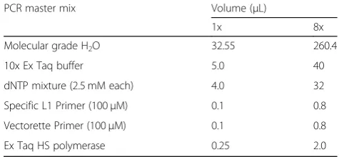
Table 5PCR master mix formulas
PCR master mix Volume (μL)
1x 8x
Molecular grade H2O 32.55 260.4
10x Ex Taq buffer 5.0 40
dNTP mixture (2.5 mM each) 4.0 32
Specific L1 Primer (100μM) 0.1 0.8
Vectorette Primer (100μM) 0.1 0.8
Ex Taq HS polymerase 0.25 2.0
Table 3Digestion master mix
Digestion master mix Volume (μL)
1x 4x
Molecular grade H2O 2.25 9.0
10x Restriction enzyme buffer 2.5 10
Restriction enzyme 1.0 4.0
14. Add 3.2μL of ligation master mix to the 6 enzyme/ vectorette tubes. Mix by gently flicking and spinning. Keep at 4 °C overnight.
Steps 15–18: Vectorette PCR (Timing: 1 h setup and 7 h runtime)
15. Inactivate ligation reactions by incubating at 65 °C for 20 min in a thermal cycler with heated lid. Pause Point:The vectorette-ligated DNA templates may be kept at 4 °C for short term or−20 °C for long term storage.
16. Prepare PCR master mix on ice for the appropriate number of samples plus excess (See Table5). Mix
by gently pipetting the entire volume 5 times and quickly spin to collect.
17. Add 42μL of PCR master mix to 8μL of each vectorette-DNA template (and to 8μL of H2O for a
no-template control). Mix by gently flicking and spinning.
Critical:Be sure to set up 6 separate PCR reactions for each of the 6 DNA-vectorette templates. Only part of the DNA template may be used, and the remainder can be kept at 4 °C for short term or
−20 °C for long term storage.
18. Run vectorette PCR program in thermal cycler with heated lid (see Table2). The program can be left to run overnight.
Table 6Data analysis using TIPseqHunter (Timing: variable)
TIPseqHunter uses genome assembly GRCh37 (hg19) and can be run with a Docker image or by using individual programs.
TIPseqHunter was developed by Java (version 7) and R (version 3.2) languages and tested under Linux operating system and is available to download at:https://github.com/fenyolab/TIPseqHunter
Docker image for TIPseqHunter was developed with the stable version of Docker Community Edition (CE) and it may work under any operating system capable to run Docker. However, we recommend the Unix-like operating systems, such as Linux and Mac OS X. Our Docker image is an alternative to the conventional TIPseqHunter program mentioned above. This image version is available at Docker Hub registry (https://hub.docker.com/) and can be downloaded with the Docker client command:docker pull galantelab/tipseqhunter. For further details, check
https://github.com/galantelab/tipseq_hunter/blob/master/README.md
Testing data and masked and bowtie-built reference genome are available to download at:http://openslice.fenyolab.org/data/tipseqhunter/test_data
Docker Prerequisite:
The Docker image works as a container and runs exactly the same TIPseqHunter program. Neither downloading of dependencies nor manually setting of software used by TIPseqHunter are required. In order to run this container you will need only need to install Docker.
For OS X:https://docs.docker.com/mac/started/
For Linux:https://docs.docker.com/linux/started/
For Windows:https://docs.docker.com/docker-for-windows/
TIPseqHunter Prerequisites:
1. At least 10GB of memory is needed if the number of sequenced read-pairs is greater than 20M.
2. Bowtie 2 alignment software (version 2.2.3 used for testing):http://bowtie-bio.sourceforge.net/bowtie2/index.shtml
3. Samtools software (latest version):http://samtools.sourceforge.net/
4. Trimmomatic software (version 0.32 used for testing):http://www.usadellab.org/cms/?page=trimmomatic
5. Java packages: sam-1.112.jar, commons-math3-3.4.1.jar, jfreechart-1.0.14.jar, jcommon-1.0.17.jar, itextpdf-5.2.1.jar, biojava3-core-3.0.1.jar 6. R packages: pROC, ggplot2, caret, e1071
Critical:BAM file has to be generated by bowtie2 alignment with "XM" tag Running TIPseqHunter:
(1) for quality control, alignment, feature selection, modeling, prediction:
./TIPseqHunterPipelineJar.sh fastq_path output_path fastq_r1 key_r1 key_r2 num_rp
Critical: Detailed information is provided in the TIPseqHunterPipelineJar.sh file. Some parameters need to be pre-set. Parameters:
fastq_path: path of the fastq files (Note: this is the only path and file name is not included)
output_folder: path of the output files (Note: this is the only path and file name is not included)
fastq_r1: read 1 file name of paired fastq files
key_r1: key word to recognize read-1 fastq file (such as "_1" is the key word for CAGATC_1.fastq fastq file)
Critical:key has to be unique in the file name
key_r2: key word to recognize read-2 fastq file and replaceable with the read-1 key word to match to read-1 file (such as "_2" is the key word for
CAGATC_2.fastq fastq file)
Critical:key has to be unique in the file name
num_rp: the total number of the read pairs in the paired fastq files (Note: it is the total number of read-pairs, i.e. either the total number of read1 or
read2 but not together.) (This number is for normalization purpose) (2) for somatic insertions:
TIPseqHunterPipelineJarSomatic.sh repred_path control_path repred_file control_file
Critical: Detailed information is provided in the TIPseqHunterPipelineJarSomatic.sh file. Some parameters need to be pre-set. Parameters:
repred_path: path of“model”folder under output folder
control_path: path "TRLocator" folder under output folder
repred_file: file with suffix ".repred" and generated from P11 in repred_path (Note: file name should be ending with ".repred".) (such as
302_T_GTCCGC.wsize100.regwsize1.minreads1.clip1.clipflk5.mindis150.FP.uniqgs.bed.csinfo.lm.l1hs.pred.txt.repred)
control_file: file with suffix“.bed”in control_path (Note: file name should be ending with ".bed".) (such as 302_N_GTGA
Steps 19–21: DNA purification and quality control (Timing: 2 h)
19. Purify PCR reactions using 1x volume of Agencourt AMPure beads. Elute in 20uL 10 mM Tris-HCL pH 8.0 and pool together.
Pause Point:Purified DNA may be kept at 4 °C for short term or−20 °C for long term storage.
20. Measure purified DNA concentration on NanoDrop.
Troubleshooting: If PCR yield is too low, restart procedure with freshly annealed vectorette
adapters, isolate fresh gDNA, or increase the initial amount of gDNA.
21. Run 2μg of purified DNA on 1.5% agarose gel. Critical:Vectorette PCR amplicons should appear as a smear on the gel averaging around 1-3 kb. (see Additional file4: Figure S1A).
Troubleshooting:The presence of a very high molecular weight smear could indicate primer-vectorette concatemer amplification. Digest 2μg of purified vectorette PCR amplicons withBstYI and run on a 1.5% agarose gel.BstYI cuts within the vectorette primer. An intense band around 50 bp indicates the presence of vectorette-primer concatemers in the PCR product (see Additional file4: Figure S1B).
Steps 22–25: DNA shearing and purification (Timing: 2 h)
22. Based on NanoDrop measurement, prepare 10μL
of 100 ng/μL purified DNA in H2O. Measure
diluted DNA concentration on Qubit.
23. Based on the Qubit measurement, dilute 1.5μg of
purified DNA in 130μL 10 mM Tris-HCL and
transfer to a Covaris microTUBE.
Critical: The Qubit is more reliable than the NanoDrop at measuring double-stranded DNA concentration.
24. Shear DNA to 300 bp using Covaris’LE220 with
recommended settings: duty factor = 30%, peak incident power = 450, cycles/burst = 200, time = 60s 25. Purify sheared DNA using QiaQuick PCR
Purification kit. Elute in 50μL H2O.
Pause Point:Sheared DNA may be kept at 4 °C for short term or−20 °C for long term storage.
QC (Optional):Run sheared DNA on Agilent 4200 TapeStation. The trace should show a peak centered around 300 bp (see Additional file3: Figure S2B).
Steps 26–28: Library preparation and quality control (Timing: 1 d)
26. Use 200 ng of sheared DNA to prepare libraries using KAPA Library Preparation Kit for Illumina
Table 7Validation of insertions through spanning PCR and Sanger sequencing (Timing: variable)
1. Design flanking primers around L1 insertion site.
Critical: Each primer should be at least 100bp away from insertion site. Avoid placing primers in repetitive DNA.
2. Set up 25uL PCR reactions with ExTaq HS following manufacturer’s instructions.
Critical: It is important to use a robust polymerase to extend through the L1 poly-A tail.
3. Use 50ng of gDNA as template.
Critical: Use the same high quality gDNA that served as starting material for TIPseq
4. Run the PCR in a thermal cycler with heated lid using a 10-minute extension for 30 cycles.
Critical:It is necessary to use an extension time long enough to amplify a full length, 6kb L1 insertion.
5. Run the PCR product on a 1% agarose gel and excise the band containing the filled allele (see Fig.3a).
Troubleshooting: If no filled band occurs, we recommend trying a 3’ L1 specific PCR. (see Table8).
6. Purify the excised DNA using Zymoclean Gel DNA Recovery Kit following the manufacturer’s instructions.
7. Sanger sequence the purified DNA using both the forward and reverse PCR primer
Table 8Validation of insertions and identification of 3’ transduction events through L1-specific 3’ PCR and Sanger sequencing (Timing: variable)
1. Design flanking primers around L1 insertion site.
Critical:Each primer should be at least 100bp away from insertion site. Avoid placing primers in repetitive DNA.
2. Set up duplicate 25uL PCR reactions with ExTaq HS following manufacturer’s instructions. Each reaction should contain one flanking primer paired with the L1 specific primer from vectorette PCR. Critical:It is important to use a robust polymerase to extend through
the L1 poly-A tail. 3. Use 50ng of gDNA as template.
Critical:Use the same high quality gDNA that served as starting material for TIPseq
4. Run the PCR in a thermal cycler with heated lid using a 60°C annealing temperature and at least a 30-second extension for 30 cycles. Critical:It is important to use a slightly higher annealing temperature
and shorter extension time to reduce the amount of off-target L1 binding and amplification.
5. Run the PCR product on a 1% agarose gel and excise the band from the successful reaction.
Critical: Only one of the two PCR reactions should produce a band. A plus stranded L1 insertion will produce a band in the reverse primer reaction, and a minus stranded L1 will produce a band in the forward primer reaction. The size of the band should equal the distance from the genomic primer to the L1 insertion site plus 150bp of L1 and polyA sequence. A band larger than expected could indicate a 3’transduction event has occurred (See Fig.3b)
6. Purify the excised DNA using Zymoclean Gel DNA Recovery Kit following the manufacturer’s instructions.
7. Sanger sequence the purified DNA using the L1 primer and either the forward or the reverse genomic primer, depending on which reaction was successful.
according to the manufacturer’s instructions without performing dual-SPRI size selection. Critical:Avoid performing library amplification. We recommend avoiding size selection, but dual-SPRI bead selection may be performed.
Pause Point:Libraries may be stored at−20 °C. 27. Perform QC on prepared libraries using qubit and
Agilent 4200 TapeStation.
Troubleshooting: If library yield is too low, restart library preparation with more sheared DNA (0.5– 1μg). If necessary, perform qPCR on prepared libraries with KAPA Library Quantification Kit to increase accuracy of quantification and pooling. 28. If necessary, appropriately pool samples to create a
multiplexed library.
Critical: Pool up to 12 samples per lane to get a minimum of 15–25 million read pairs per sample. Troubleshooting:Performing qPCR on prepared libraries with KAPA Library Quantification Kit prior to pooling may result in a more balanced sequencing output.
Steps 29: Illumina deep sequencing (Timing: 1–4 d)
29. Sequence 200pM of pooled library with 20% PhiX on Illumina HiSeq4000, 150 cycles, paired end. If necessary, demultiplex raw reads.
Steps 30–31: Data analysis and validation (Timing: Variable)
30. Analyze data using TIPseqHunter (see Table6).
Troubleshooting:If the data contain a large amount of overlapping read pairs, use Pippin prep selection after pooling (step 28) to remove fragments under 400 bp. 31. Perform PCR validation and Sanger sequencing
(see Tables 7 and 8)
Timing
Steps 1–5, vectorette adapter annealing: 2 h Steps 6–9, genomic DNA digestion: 1 h setup and overnight incubation
Steps 10–14, vectorette adapter ligation: 3 h setup and overnight incubation
Steps 15–18, vectorette PCR: 1 h setup and 7 h runtime Steps 19–21, DNA purification and quality control: 2 h Note: Waiting and processing time varies when sending PCR amplicons to a sequencing core facility.
Steps 22–25, DNA shearing and purification: 1 h Steps 26–28, library preparation and quality control: 1 d Step 29, Illumina deep sequencing: 1–4 days
Steps 30–31, Data analysis and validation: variable Table6, Data analysis using TIPseqHunter: variable Table7, Validation of insertions through spanning PCR and Sanger sequencing: variable
Table8, Validation of insertions and identification of 3′ transduction events through L1-specific 3’PCR and Sanger sequencing: variable
Note: Sequencing, analysis, and validation time will vary depending on the number of samples being processed and number of insertions to validate.
Troubleshooting
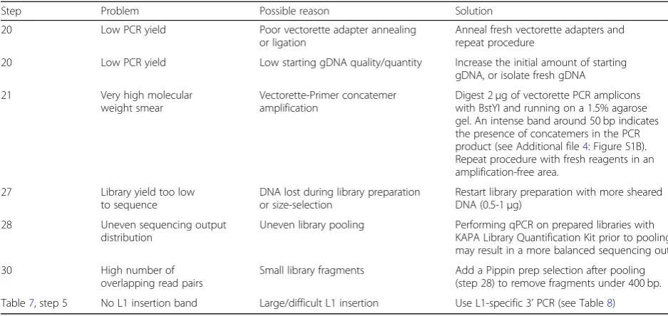
See Table9for troubleshooting information. Table 9Troubleshooting table
Step Problem Possible reason Solution
20 Low PCR yield Poor vectorette adapter annealing or ligation
Anneal fresh vectorette adapters and repeat procedure
20 Low PCR yield Low starting gDNA quality/quantity Increase the initial amount of starting gDNA, or isolate fresh gDNA
21 Very high molecular weight smear
Vectorette-Primer concatemer amplification
Digest 2μg of vectorette PCR amplicons with BstYI and running on a 1.5% agarose gel. An intense band around 50 bp indicates the presence of concatemers in the PCR product (see Additional file4: Figure S1B). Repeat procedure with fresh reagents in an amplification-free area.
27 Library yield too low to sequence
DNA lost during library preparation or size-selection
Restart library preparation with more sheared DNA (0.5-1μg)
28 Uneven sequencing output distribution
Uneven library pooling Performing qPCR on prepared libraries with KAPA Library Quantification Kit prior to pooling may result in a more balanced sequencing output.
30 High number of overlapping read pairs
Small library fragments Add a Pippin prep selection after pooling (step 28) to remove fragments under 400 bp.
Additional files
Additional file 1:Table S1.Scaled-down reaction sizes. (XLSX 13 kb) Additional file 2:Table S2.Design of the vectorette oligo and primer sequences. (XLSX 12 kb)
Additional file 3:Figure S2.DNA size distributions during TIPseq.a.
An Agilent TapeStation image of two samples of purified vectorette PCR DNA is shown with amplicons averaging 1-3 kb. The protocol does not require running samples on TapeStation after vectorette PCR, but this image is included to illustrate the size range.b.The second TapeStation image shows the samples after DNA shearing. The average size distribution for the sheared DNA should be approximately 300 bp.c.As a final quality control, samples should be run on the TapeStation after library prep is completed. This image shows the increase in size from the Illumina adapters and an average library size around 400 bp. (PDF 952 kb)
Additional file 4:Figure S1.Vectorette PCR amplicons quality control.
a.Electrophoresis of vectorette PCR amplicons. The gel image shows five lanes: [L] 2-log ladder (NEB) [1], 2μg purified PCR amplicons [2], 2μg purified PCR amplicons digested withBstYI [3], 2μg purified PCR amplicons
‘contaminated’with concatemers [4], 2μg purified PCR amplicons digested withBstYI showing concatemer band at ~ 50 bp. A good vectorette PCR will present as a smear of amplicons averaging 1-3 kb (lane 1). A very high molecular weight smear could indicate contamination (lane 3).b.Schematic of possible vectorette-primer concatemer. Digestion of the amplicons with
BstYI, which cuts inside the vectorette primer sequence, will produce a visible band at ~ 50 bp if concatemers are in the PCR product. (PDF 2479 kb)
Additional file 5:Table S3.Retrotransposon primer sequences. (XLSX 8 kb)
Abbreviations
L1Hs:Homo sapiens-specific L1; LINE-1, L1: Long interspersed element-1; TIP: Transposon insertion profiling
Acknowledgements
The authors thank Peilin Shen, Anna Schneider, and Pragathi Achanta for technical assistance and valuable discussions while developing TIPchip and TIPseq; and Nemanja Rodić, Christine Iacobuzio-Donahue, Alfredo Quiñones-Hinojosa, Tian-Li Wang, and Ie-Ming Shih for materials and clinical expertise related to somatic retrotransposition studies in human cancers.
Funding
This work has been supported by R01CA163705, R01GM124531, and grants from the Sol Goldman Pancreatic Cancer Research Center and the Maryland Cigarette Restitution Fund (to KHB) and P50GM107632 (to JDB and KHB).
Availability of data and materials
Data sharing not applicable to this article as no datasets were generated in the current study. Example TIPseq datasets can be obtained on NCBI BioProject under accession numbers PRJNA324255, PRJNA319653, and PRJNA319649.
Authors’contributions
KHB and JDB guided the study. JPS, CRLH, and LMP developed and optimized the procedure. SR and AH optimized library preparation and sequencing. ZT, MG, and DF developed the computational analysis pipeline and software. FORR, TLAM, and PAFG created the Docker image. JPS and KHB wrote the paper. All authors read and approved the final manuscript.
Ethics approval and consent to participate
Not applicable.
Consent for publication
Not applicable.
Competing interests
The authors declare that they have no competing interests.
Publisher’s Note
Springer Nature remains neutral with regard to jurisdictional claims in published maps and institutional affiliations.
Author details
1Department of Pathology, Johns Hopkins University School of Medicine, Baltimore, MD 21205, USA.2McKusick–Nathans Institute of Genetic Medicine, Johns Hopkins University School of Medicine, Baltimore, MD 21205, USA. 3Department for Biochemistry and Molecular Pharmacology, NYU Langone Health, New York, NY 10016, USA.4Institute for Systems Genetics, NYU Langone Health, New York, NY 10016, USA.5Centro de Oncologia Molecular, Hospital Sírio-Libanês, São Paulo, Brazil.6Departamento de Bioquímica, Instituto de Química, Universidade de São Paul, São Paulo, Brazil.7Genome Technology Center, Division of Advanced Research Technologies, NYU Langone Health, New York, NY, USA.
Received: 23 October 2018 Accepted: 14 January 2019
References
1. Lander ES, Linton LM, Birren B, Nusbaum C, Zody MC, Baldwin J, Devon K, Dewar K, Doyle M, FitzHugh W, et al. Initial sequencing and analysis of the human genome. Nature. 2001;409(6822):860–921.
2. Skowronski J, Fanning TG, Singer MF. Unit-length line-1 transcripts in human teratocarcinoma cells. Mol Cell Biol. 1988;8(4):1385–97.
3. Sheen FM, Sherry ST, Risch GM, Robichaux M, Nasidze I, Stoneking M, Batzer MA, Swergold GD. Reading between the LINEs: human genomic variation induced by LINE-1 retrotransposition. Genome Res. 2000;10(10):1496–508. 4. Brouha B, Schustak J, Badge RM, Lutz-Prigge S, Farley AH, Moran JV,
Kazazian HH Jr. Hot L1s account for the bulk of retrotransposition in the human population. Proc Natl Acad Sci U S A. 2003;100(9):5280–5. 5. Beck CR, Collier P, Macfarlane C, Malig M, Kidd JM, Eichler EE, Badge RM,
Moran JV. LINE-1 retrotransposition activity in human genomes. Cell. 2010; 141(7):1159–70.
6. Philippe C, Vargas-Landin DB, Doucet AJ, van Essen D, Vera-Otarola J, Kuciak M, Corbin A, Nigumann P, Cristofari G. Activation of individual L1 retrotransposon instances is restricted to cell-type dependent permissive loci. Elife. 2016;5:e13926.
7. Deininger P, Morales ME, White TB, Baddoo M, Hedges DJ, Servant G, Srivastav S, Smither ME, Concha M, DeHaro DL, et al. A comprehensive approach to expression of L1 loci. Nucleic Acids Res. 2016;45:e31. 8. Xing J, Zhang Y, Han K, Salem AH, Sen SK, Huff CD, Zhou Q, Kirkness EF,
Levy S, Batzer MA, et al. Mobile elements create structural variation: analysis of a complete human genome. Genome Res. 2009;19(9):1516–26. 9. Huang CR, Schneider AM, Lu Y, Niranjan T, Shen P, Robinson MA, Steranka
JP, Valle D, Civin CI, Wang T, et al. Mobile interspersed repeats are major structural variants in the human genome. Cell. 2010;141(7):1171–82. 10. Stewart C, Kural D, Stromberg MP, Walker JA, Konkel MK, Stutz AM, Urban
AE, Grubert F, Lam HY, Lee WP, et al. A comprehensive map of mobile element insertion polymorphisms in humans. PLoS Genet. 2011;7(8):e1002236. 11. Sudmant PH, Rausch T, Gardner EJ, Handsaker RE, Abyzov A, Huddleston J,
Zhang Y, Ye K, Jun G, Hsi-Yang Fritz M, et al. An integrated map of structural variation in 2,504 human genomes. Nature. 2015;526(7571):75–81. 12. Dewannieux M, Esnault C, Heidmann T. LINE-mediated retrotransposition of
marked Alu sequences. Nat Genet. 2003;35(1):41–8.
13. Konkel MK, Walker JA, Hotard AB, Ranck MC, Fontenot CC, Storer J, Stewart C, Marth GT, Genomes C, Batzer MA. Sequence analysis and characterization of active human Alu subfamilies based on the 1000 genomes pilot project. Genome Biol Evol. 2015;7(9):2608–22.
14. Witherspoon DJ, Xing J, Zhang Y, Watkins WS, Batzer MA, Jorde LB. Mobile element scanning (ME-scan) by targeted high-throughput sequencing. BMC Genomics. 2010;11:410.
15. Witherspoon DJ, Zhang Y, Xing J, Watkins WS, Ha H, Batzer MA, Jorde LB. Mobile element scanning (ME-scan) identifies thousands of novel Alu insertions in diverse human populations. Genome Res. 2013;23(7):1170–81. 16. Hancks DC, Goodier JL, Mandal PK, Cheung LE, Kazazian HH Jr.
Retrotransposition of marked SVA elements by human L1s in cultured cells. Hum Mol Genet. 2011;20(17):3386–400.
17. Iskow RC, McCabe MT, Mills RE, Torene S, Pittard WS, Neuwald AF, Van Meir EG, Vertino PM, Devine SE. Natural mutagenesis of human genomes by endogenous retrotransposons. Cell. 2010;141(7):1253–61.
19. Tubio JM, Li Y, Ju YS, Martincorena I, Cooke SL, Tojo M, Gundem G, Pipinikas CP, Zamora J, Raine K, et al. Mobile DNA in cancer. Extensive transduction of nonrepetitive DNA mediated by L1 retrotransposition in cancer genomes. Science. 2014;345(6196):1251343.
20. Helman E, Lawrence MS, Stewart C, Sougnez C, Getz G, Meyerson M. Somatic retrotransposition in human cancer revealed by whole-genome and exome sequencing. Genome Res. 2014;24(7):1053–63.
21. Solyom S, Ewing AD, Rahrmann EP, Doucet T, Nelson HH, Burns MB, Harris RS, Sigmon DF, Casella A, Erlanger B, et al. Extensive somatic L1 retrotransposition in colorectal tumors. Genome Res. 2012;22(12):2328–38. 22. Rodic N, Steranka JP, Makohon-Moore A, Moyer A, Shen P, Sharma R,
Kohutek ZA, Huang CR, Ahn D, Mita P, et al. Retrotransposon insertions in the clonal evolution of pancreatic ductal adenocarcinoma. Nat Med. 2015; 21(9):1060–4.
23. Tang Z, Steranka JP, Ma S, Grivainis M, Rodic N, Huang CR, Shih IM, Wang TL, Boeke JD, Fenyo D, et al. Human transposon insertion profiling: analysis, visualization and identification of somatic LINE-1 insertions in ovarian cancer. Proc Natl Acad Sci U S A. 2017;114(5):E733–40.
24. Baillie JK, Barnett MW, Upton KR, Gerhardt DJ, Richmond TA, De Sapio F, Brennan PM, Rizzu P, Smith S, Fell M, et al. Somatic retrotransposition alters the genetic landscape of the human brain. Nature. 2011;479(7374):534–7. 25. Shukla R, Upton KR, Munoz-Lopez M, Gerhardt DJ, Fisher ME, Nguyen T,
Brennan PM, Baillie JK, Collino A, Ghisletti S, et al. Endogenous retrotransposition activates oncogenic pathways in hepatocellular carcinoma. Cell. 2013;153(1):101–11.
26. Upton KR, Gerhardt DJ, Jesuadian JS, Richardson SR, Sanchez-Luque FJ, Bodea GO, Ewing AD, Salvador-Palomeque C, van der Knaap MS, Brennan PM, et al. Ubiquitous L1 mosaicism in hippocampal neurons. Cell. 2015; 161(2):228–39.
27. Carreira PE, Ewing AD, Li G, Schauer SN, Upton KR, Fagg AC, Morell S, Kindlova M, Gerdes P, Richardson SR, et al. Evidence for L1-associated DNA rearrangements and negligible L1 retrotransposition in glioblastoma multiforme. Mob DNA. 2016;7:21.
28. Sanchez-Luque FJ, Richardson SR, Faulkner GJ. Retrotransposon capture sequencing (RC-Seq): a targeted, high-throughput approach to resolve somatic L1 Retrotransposition in humans. Methods Mol Biol. 2016;1400:47–77. 29. Nguyen THM, Carreira PE, Sanchez-Luque FJ, Schauer SN, Fagg AC,
Richardson SR, Davies CM, Jesuadian JS, Kempen MHC, Troskie RL, et al. L1 retrotransposon heterogeneity in ovarian tumor cell evolution. Cell Rep. 2018;23(13):3730–40.
30. Ewing AD, Kazazian HH Jr. High-throughput sequencing reveals extensive variation in human-specific L1 content in individual human genomes. Genome Res. 2010;20(9):1262–70.
31. Evrony GD, Cai X, Lee E, Hills LB, Elhosary PC, Lehmann HS, Parker JJ, Atabay KD, Gilmore EC, Poduri A, et al. Single-neuron sequencing analysis of L1 retrotransposition and somatic mutation in the human brain. Cell. 2012; 151(3):483–96.
32. Evrony GD, Lee E, Mehta BK, Benjamini Y, Johnson RM, Cai X, Yang L, Haseley P, Lehmann HS, Park PJ, et al. Cell lineage analysis in human brain using endogenous retroelements. Neuron. 2015;85(1):49–59.
33. Doucet-O'Hare TT, Rodic N, Sharma R, Darbari I, Abril G, Choi JA, Young Ahn J, Cheng Y, Anders RA, Burns KH, et al. LINE-1 expression and
retrotransposition in Barrett's esophagus and esophageal carcinoma. Proc Natl Acad Sci U S A. 2015;112(35):E4894–900.
34. Doucet TT, Kazazian HH Jr. Long interspersed element sequencing (L1-Seq): a method to identify somatic LINE-1 insertions in the human genome. Methods Mol Biol. 2016;1400:79–93.
35. Doucet-O'Hare TT, Sharma R, Rodic N, Anders RA, Burns KH, Kazazian HH Jr. Somatically acquired LINE-1 insertions in Normal esophagus undergo clonal expansion in esophageal squamous cell carcinoma. Hum Mutat. 2016;37(9):942–54.
36. Rahbari R, Badge RM. Combining amplification typing of L1 active subfamilies (ATLAS) with high-throughput sequencing. Methods Mol Biol. 2016;1400:95–106.
37. Evrony GD, Lee E, Park PJ, Walsh CA. Resolving rates of mutation in the brain using single-neuron genomics. Elife. 2016;5:e12966.
38. Scott EC, Gardner EJ, Masood A, Chuang NT, Vertino PM, Devine SE. A hot L1 retrotransposon evades somatic repression and initiates human colorectal cancer. Genome Res. 2016;26(6):745–55.
39. Pradhan B, Cajuso T, Katainen R, Sulo P, Tanskanen T, Kilpivaara O, Pitkanen E, Aaltonen LA, Kauppi L, Palin K. Detection of subclonal L1 transductions in
colorectal cancer by long-distance inverse-PCR and Nanopore sequencing. Sci Rep. 2017;7(1):14521.
40. Ewing AD, Kazazian HH Jr. Whole-genome resequencing allows detection of many rare LINE-1 insertion alleles in humans. Genome Res. 2011;21(6):985–90.
41. Gardner EJ, Lam VK, Harris DN, Chuang NT, Scott EC, Pittard WS, Mills RE, Genomes Project C, Devine SE. The Mobile Element Locator Tool (MELT): population-scale mobile element discovery and biology. Genome Res. 2017; 27(11):1916–29.
42. Wheelan SJ, Scheifele LZ, Martinez-Murillo F, Irizarry RA, Boeke JD. Transposon insertion site profiling chip (TIP-chip). Proc Natl Acad Sci U S A. 2006; 103(47):17632–7.
43. Huang CR, Burns KH, Boeke JD. Active transposition in genomes. Annu Rev Genet. 2012;46:651–75.
44. Achanta P, Steranka JP, Tang Z, Rodic N, Sharma R, Yang WR, Ma S, Grivainis M, Huang CR, Schneider AM, et al. Somatic retrotransposition is infrequent in glioblastomas. Mob DNA. 2016;7:22.