Estimation of infiltration models parameters and their comparison to
simulate the onsite soil infiltration characteristics
Hafiz Umar Farid
1*,
Zahid Mahmood-Khan
1,
Ijaz Ahmad
2,
Aamir Shakoor
1,
Muhammad Naveed Anjum
3,
Muhammad Mazhar Iqbal
4,
Muhammad Mubeen
5,
Muhammad Asghar
1(1. Department of Agricultural Engineering, Bahauddin Zakariya University, Multan-Pakistan;
2. Center of Excellence in Water Resources Engineering (CEWRE), University of Engineering and Technology, Lahore-Pakistan;
3. Division of Hydrology Water-Land Resources in Cold and Arid Regions, Cold and Arid Region Environmental and Engineering Institute, Chinese Academy of Sciences, Lanzhou 730000, China;
4. Graduate School of Water Resources, Sungkyunkwan University, Suwon-si 2066, Korea; 5. Department of Environmental Sciences, COMSATS Institute of Information Technology, Vehari-Pakistan)
Abstract: Detailed knowledge about soil characteristics and site-specific final steady infiltration rate could help to increase the irrigation water use efficiency and decrease water losses in agricultural system. The experiments were conducted on Agricultural Research Farm of Bahauddin Zakariya University, Multan, Pakistan during 2016. The cumulative infiltration depth was measured using double ring infiltrometer at selected six points of the study area. Most commonly used infiltration models such as Kostikov’s, Philip’s and Horton’s were fitted to the field infiltration data for determination of model parameters and to find the best fit model for the study area. Kostikov’s infiltration model’s parameters such as empirical constant ‘c’ and infiltration decay constants ‘k’ were obtained in the ranges of 0.140-0.290 and 0.307-0.433, respectively. Philip’s infiltration model’s parameters such as sorptivity ‘S’ and conductivity constant ‘A’ were found in the ranges of 0.167-0.288 cm/min1/2 and –0.001 to –0.009 cm/min, respectively. Similarly, the Horton’s model’s ‘parameter ‘k’ was obtained in the range of –1.619 to –1.238. The value of infiltration capacity at onset of infiltration (fo) was obtained as 1.744 to 3.491 for all the six points. The analysis showed that the infiltration models using the estimated parameters have satisfactory prediction capability at all the selected points. Horton’s model provided the lowest mean values for RMSE (0.235) and highest mean values for ME (94%); and the lowest mean values for MPD (0.127). This indicated that infiltration can be well-described by the Horton’s model at the selected site.
Keywords: infiltration characteristics, infiltration models, parameters estimation, perdition capability
DOI: 10.25165/j.ijabe.20191203.4015
Citation: Farid H U, Mahmood-Khan Z, Ahmad I, Shakoor A, Anjum M N, Iqbal M M, et al. Estimation of infiltration models parameters and their comparison to simulate the onsite soil infiltration characteristics. Int J Agric & Biol Eng, 2019; 12(3): 84–91.
1 Introduction
1Soil water is an insignificant fraction of the total available water on the planet earth, but it is considered as the most important one because it plays an important role in the availability of water to plants under various soil conditions[1-4]. The major inputs to the
Received date: 2017-11-30 Accepted date: 2019-03-10
Biographies: Zahid Mahmood-Khan, PhD, Associate Professor, research interest: water engineering and management and water quality, Email: [email protected]; Ijaz Ahmad, PhD, Assistant Professor, research interest: hydrology and watershed modelling, Email: [email protected]; Aamir Shakoor, PhD, Assistant Professor, research interest: water saving and irrigation modeling, Email: [email protected]; Muhammad Naveed Anjum, PhD, research interest: hydrology and watershed modelling, Email: naveedwre@ yahoo.com; Muhammad Mazhar Iqbal, PhD, research interest: hydrology and river quality modelling, Email: [email protected]; Muhammad Mubeen, PhD, Assistant Professor, research interest: irrigation and crop modelling, Email: [email protected]; Muhammad Asghar,
Graduate student, Design Engineer, research interest: irrigation and water application, Email: [email protected].
*Corresponding author: Hafiz Umar Farid, PhD, Assistant Professor, research interest: hydrology and precision water management, Email: hufarid@ bzu.edu.pk. Department of Agricultural Engineering, Bahauddin Zakariya University, Multan. Tel/Fax: +92-65-9210298.
soil water are the rainfall and irrigation[5,6]. The rainfall and irrigation water can be divided into two major parts. One part goes to the sea as surface runoff through overland flow and stream channels and other part goes initially into the soil through the infiltration[2,7]. Infiltration is the process by which water moves into the soil from the ground surface. It is considered as one of the most important components of the hydrological cycle[8-11]. Furthermore, during the application of water to the agricultural field, infiltration is one of the most critical processes to control the surface irrigation uniformity and increased irrigation efficiency[12,13]. Infiltration is a key dynamic process which can be considered for scheduling, design, management and optimization of irrigation system[14-17]. Due to fundamental role of infiltration in hydrology, irrigation and agriculture systems, it has received a great attention by the soil and water scientists[4,16-18]. Oku and Aiyelari[19] reported that soil infiltration characteristics can be quantified by fitting the field infiltration data to the model infiltration. Similarly, detailed knowledge about the soil infiltration rate and characteristics increases the irrigation water use efficiency and decreases water losses[10,20].
determine the soil infiltration rate and characteristics[21,22]. These infiltration models have been thoroughly and comprehensively reviewed, presented and summarized[5,22-24]. All models are not applicable to all types of soils because of the dependency of infiltration rate on soil texture[25,26]. Several research studies have been conducted to estimate the parameters of infiltration models and to validate these models for different soil conditions[20,21,27,28]. Igbadun and Idris[27] investigated the Kostiakov’s, Kostiakov- Lewis, modified Kostiakov and Philip’s infiltration models at the flood plain in Zango village, Samaru Zaria Nigeria to determine the water infiltration into the soil. The results indicated that the tested four models have good abilities to predict infiltration data. However, Kostokov’s and modified Kostikov’s had better fitness to the measured values. Oku and Aiyelari[20] reported that Philip’s model provided better performance than Kostiakov’s model for prediction of infiltration into Inceptisols in the forest humid zone of Nigeria. The satisfactory performance of Philip’s model for prediction of water infiltration in the soils of Aba, Abia state Nigeria has also been observed by Adindu et al.[28] and Musa et al.[1] stated that Kostikov’s model showed a better performance than those of Philip’s and Horton’s models based on the fitted infiltration equations to the soil of farm site of the Federal University of Technology, Minna, Nigeria. The Horton’s models have also been suggested by Roohian et al.[29] to give good estimations of final infiltration rate under the given soil textural conditions in Taleghan watershed of Tehran Province, Iran. Similarly, Mbagwu[30] reported that Philip’s model would always fail to predict infiltration data if the assumptions of the model are not met. Therefore, the need for continuous in-depth and field specific study of the applicability of infiltration equations cannot be over-emphasized because models’ parameters and performance vary from point to point and vary with time. Keeping in view the above referred studies, the parameters of three infiltration models such as Kostikov’s, Philip’s and Horton’s in a silty clay soil of the Agricultural Research Farm, Bahauddin Zakariya University, Multan were determined, and the performances of selected infiltration models were evaluated to test the competence of these models to predict the cumulative infiltration depths.
2 Materials and methods
2.1 Characteristics of the study area
The experiments were conducted at Agricultural Research Farm of Bahauddin Zakariya University, Multan, Pakistan (longitude 71.47°, latitude 30.21°, elevation 122 m above mean sea level) during 2016. The study area has arid climate with an average annual rainfall of 200 mm. The maximum temperature of 23.4°C and minimum temperature of 4.8°C were recorded during the winter. Similarly, the maximum temperature of 47°C and minimum temperature of 26°C were observed during the summer. Wheat is the major crop of the study area. Six points were selected in the study area so that each point had minimum differences in soil properties. All the points were located within 300 m radius. Each selected point was approximately 50 m apart. The soil of the selected points was measured as silty clay. According to the textural triangle provided by the US Geological Department, all the selected points have the same soil texture.
2.2 Soil sampling
A total of 24 soil samples were collected from six selected points at 0-30 cm depth of soil. These soil samples were analyzed in the Soil Mechanic Laboratory of the Agricultural Engineering Department, Bahauddin Zakariya University, Multan to determine
soil texture and other properties. At each point, undisturbed soil samples of cores of 5 cm height and diameter were collected to measure saturated hydraulic conductivity (Ks), initial moisture contents, soil bulk density, and total porosity. The Walkley-Black wet oxidation (Equations (1) and (2)) and Bouyoucos Hydrometer methods were used to determine the organic matter and soil texture, respectively[31,32]. The soil bulk density was calculated using the core method[33]. The Ks, total porosity, and initial moisture contents were measured using constant head permeability (Equation (3)), saturated moisture contents and gravimetric methods, respectively[34].
2
( ) 12
100%
4000
B S Mof Fe C
g of soil
+
− × ×
= ×
× (1)
where, B is Fe2+ solution used to titrate blank, mL; S is Fe2+solution used to titrate sample, mL; 12/4000 represents milliequivalent weight of C, g.
1.72 100%
0.58
total carbon
Organic Matter= × × (2)
Q L Ks
A h t
× =
× × (3)
where, Ks is saturated hydraulic conductivity, cm/s; Q is discharge, cm3/s; L is length of the specimen, cm; A is cross sectional area of the specimen, cm2; h is constant head causing flow, cm; t is time, s.
2.3 Infiltration measurement
The double ring infiltrometer, with 60 cm outer diameter and 25 cm inner diameters rings were installed in the soil to measure field infiltration. The double ring infiltrometer was driven to a depth of 10 cm into the soil maintaining the level of each. The measuring gauge was fixed inside the inner ring to record the amount of water infiltrated into the soil. The readings were taken at an interval of 10, 30, 60, 90, 120, 150 and 180 min. An average infiltration head of 15 cm was maintained during these time intervals. Similarly, infiltration measurement was made at each selected point (Point-1 to Point-6). The experiment remained continuous; the steady state infiltration rate was reached. After reaching the steady state infiltration rate, the experiment was stopped and the infiltration rate, cm/min, and cumulative infiltration depth, cm, were calculated.
2.4 Determination of infiltration model parameters
Several models that simplify the concepts involved in the infiltration process have been developed for field applications. In the present study, most commonly used infiltration models such as Kostikov[35], Philip[36] and Horton[37] models were selected for evaluation. The field experimental data were used to evaluate these infiltration models and to obtain numerical values of the model’s parameters. The brief description of these models and experimental setup are given below.
2.4.1 Kostikov’s model
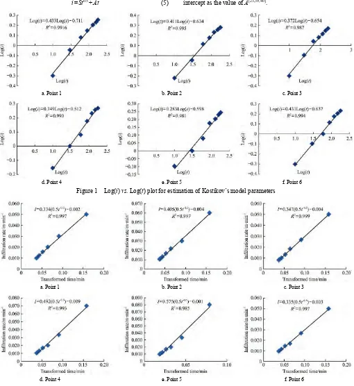
Kostikov[35] proposed a simple empirical infiltration model based on the data observed in the field or laboratory. The model relates the infiltration to as a power function as described in Equation (4):
i=ctk (4)
(Figure 1). The slope of the plotted line gave values of parameter
c and the intercept gave the value of logk. The value of k was estimated by taking anti-logk[38].
2.4.2 Philip’s model
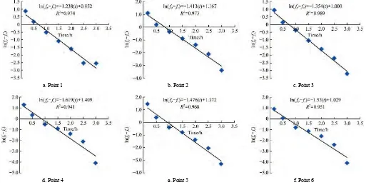
Philip[36] proposed an empirical model for infiltration by truncating the series of solution from a pounded surface. The resulting Equation (5) is expressed as:
i = St0.5 + At (5)
where, i is cumulative infiltration, cm; S is sorptivity, cm/min1/2; t is time of infiltration, min, and A is parameters related to saturated hydraulic conductivity, cm/min. The estimation of S and A values were made by fitting the infiltration rate, cm/min, data against the transformed time (1/2t0.5) by the least square regression for all the six data points (Figure 2). The resulting plot gives the straight line. The slope of the straight line gives the value of S and intercept as the value of A[23,39,40].
a. Point 1 b. Point 2 c. Point 3
d. Point 4 e. Point 5 f. Point 6
Figure 1 Log(i) vs. Log(t) plot for estimation of Kostikov’s model parameters
a. Point 1 b. Point 2 c. Point 3
d. Point 4 e. Point 5 f. Point 6
Figure 2 Infiltration rate vs. transformed time plot for estimation of Philip’s model parameters 2.4.3 Horton’s model
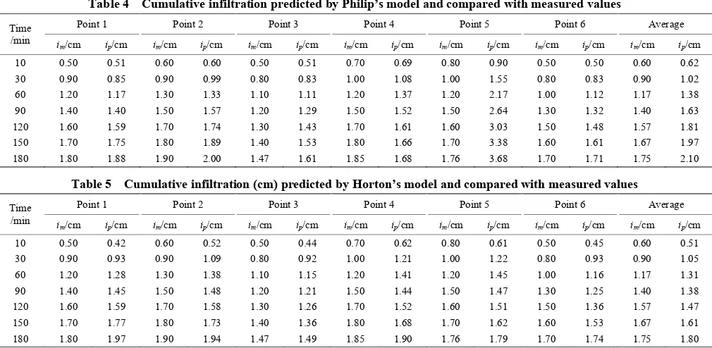
Horton[37] derived the relationship using the work and energy principle for estimation of infiltration rates. The relationship (Equation (6)) is given as:
fp = fc +( fo – fc)e-k (6)
where, fpisinfiltration capacity of soil at time (t); fcisthe constant
infiltration capacity when time approaches infinity; fois the
infiltration capacity at onset of infiltration and kis constant dependent on soil and initial soil and water conditions. The parameters of Horton’s model such as fo and k were determined by
subtracting the value of fc from experimental values of fp. The
time (t) (Figure 3). The resulting graph is a straight line and slope of the line gave the value of k. The base value for parameters k is equal to a negative slope and the initial infiltration capacity (fo) was
calculated using the fo – fc = eintercept as reported by Turner [41].
The estimated values of infiltration model’s parameters were incorporated to the model equations for all the three models to simulate cumulative infiltration depth for each point. The field data were compared with the model’s simulated data to evaluate the capability of the model to simulate cumulative infiltration.
2.5 Model selection
Several approaches have been used by different researchers for selection of suitable models for the experimental fields. Minimizing the difference between the observed and simulated values is one of the simplest approaches to find the best fit
infiltration model. Similarly, the coefficient of determination (R2) was used by Machiwal et al.[40] as a criterion to compare the infiltration models. Haghighi et al.[42] selected the best model for infiltration data using the coefficient of determination (R2) and root mean square error (RMSE) parameters. To compare the Kostikov’s and Philip’s models, the absolute mean difference (AMD) and coefficient of determination (R2) have also been used by Mudiare et al.[43] Igbadun and Idris[27] used the coefficient of efficiency to examine the suitability of infiltration model. Keeping in view the above referred research studies, the best infiltration model was selected using the root mean square error (RMSE), model efficiency (ME) and mean percent difference (MPD) as reported by Nash and Sutcliffe[44], Fang et al.[45], Bakhsh et al.[46] and Farid et al.[47]
a. Point 1 b. Point 2 c. Point 3
d. Point 4 e. Point 5 f. Point 6
Figure 3 ln(fp–fc) vs. time plot for estimation of Horton’s model parameters
3 Results and discussions
Soil properties of the experimental site showed little variability among the six selected points (Table 1). Soil textures were predominantly silty clay having clay fraction of 45%-50% and silt fraction of 41%-46%. Soil electrical conductivity (EC) was measured using soil saturated paste extract methodology and it was ranged from 0.68 dS/m to 0.98 dS/m[48]. The values of EC greater than 4 dS/m indicated the salinity problems[49]. However, the EC of soil at the study area within the permissible limit. Thus, soils of the experimental site do not have salinity problems. Bulk density values were ranged from 1.30 g/cm3 to 1.38 g/cm3 and soil porosity values were ranged from 0.49 to 0.56. Similarly, the saturated hydraulic conductivity and organic matter were ranged from 0.57-0.63 µm/s and 0.61%-0.68%, respectively. Overall analysis indicated that these points had homogenous soil and similar soil surface conditions.
3.1 Models estimated parameter
Derived parameters for the three infiltration model’s (Kostikov’s, Philip’s, Horton’s) parameters appeared similar to those reported in the literature (Table 2). Kostikov’s infiltration model’s parameters such as the values of empirical constant ‘c’
were estimated in the range of 0.140-0.290 and the values of infiltration decay constants ‘k’ were obtained in the range of 0.307-0.433. The values of infiltration decay constant ‘k’ were in accordance to the theory of infiltration that described the values to be positive and always less than unity. It has also been reported that most values of these parameters lie between the 0.2-0.9[2,50,51]. The Philip’s infiltration model parameters such as sorptivity ‘S’ values were found in the range of 0.167-0.288 cm/min1/2 and conductivity constant ‘A’ values were obtained as –0.001 to –0.009 cm/min for all the six points. The estimated values for sorptivity ‘S’ were in close agreement to the values as reported by Leao and Perfect[52]. Azuka et al.[53] described the high variability of these parameters along the toposequence. Similarly, Horton’s model’s parameters such as constant ‘k’ was determined in the range of –1.619 to –1.238. The values of infiltration capacity at onset of infiltration ‘fo’ were obtained as 1.744 to 3.491 for all the
Table 1 Soil properties of experimental site
Points Sand /% Silt /% Clay /% Textural class /dS·mEC -1 Bulk density/g·cm-3 Porosity
1 10 43 47 Silty clay 0.98 1.36 0.54 2 8 44 48 Silty clay 0.75 1.30 0.49 3 11 44 45 Silty clay 0.83 1.34 0.51 4 8 42 50 Silty clay 0.88 1.35 0.55 5 12 41 47 Silty clay 0.68 1.38 0.51 6 9 46 45 Silty clay 0.79 1.33 0.56 Table 2 Estimated values of infiltration models’ parameters
Points
Kostikove’s model
i=ctk
Philip’s model
i=St0.5+At
Horton’s model
fp=(fo–fc)e-kt+fc
c k S A k fo
1 0.140 0.433 0.167 –0.002 –1.238 1.744 2 0.197 0.411 0.203 –0.004 –1.413 2.612 3 0.184 0.372 0.174 –0.004 –1.530 2.198 4 0.290 0.307 0.246 –0.009 –1.354 2.118 5 0.223 0.399 0.288 –0.001 –1.619 3.491 6 0.195 0.431 0.168 –0.003 –1.354 3.343 3.2 Prediction of cumulative infiltration depth
Cumulative infiltrations predicted by Kostikov’s model were like the measured values in the field for point 1 to point 6 (Table 3). It was observed that the predicted cumulative infiltration depths were in close agreement with the measured ones from the field for all the points. However, Kostikov’s model under-predicted for
the Point 1 to Point 5 and over-predicted at Point 6 for all the experimental times. Similarly, the average cumulative infiltration depth was under-predicted by Kostikov’s model.
The predicted cumulative infiltration depths by Philip’s model were compared with the measured field infiltration data (Table 4). The analysis indicated that the predicted infiltration values were close to the measured values for all the points except Point 5. The model predicted infiltration depth at the initial stage up to 10 min was in close agreement to the measured infiltration depth at Point 5 and after 10 min of the period, the model over-predicted the infiltration depth which slightly differed from other measured values at Point 5. Difference in predicted and measured soil infiltration depths at Point 5 may be due to highly compacted soils at that point because Ks values decreased significantly as the compaction increased. Compact soil affects the soil physical quality, pore size distribution, Ks and capillary fringe thickness[11]. However, the average measured and predicted values for all the points were in an acceptable range (Table 4). The predicted cumulative infiltration depth by the Horton’s model also agreed with that of measured field data for all the selected points (Table 5). On average, Horton’s model under-predicted at the initial stage up to 10 min, over-predicted at 30 min and 180 min of the period. The mix behavior was observed at 60, 90, 120 and 150 min of the period for all the data points. Overall analysis showed that these infiltration models using the estimated parameters have satisfactory prediction capability at all the selected points because the model performance indicators were in acceptable limits as discussed in the subsequent section.
Table 3 Cumulative infiltration predicted by Kostikov’s model and compared with measured values
Time /min
Point 1 Point 2 Point 3 Point 4 Point 5 Point 6 Average
im/cm ip/cm im/cm ip/cm im/cm ip/cm im/cm ip/cm im/cm ip/cm im/cm ip/cm im/cm ip/cm 10 0.5 0.40 0.60 0.51 0.50 0.43 0.70 0.59 0.80 0.56 0.50 0.56 0.60 0.51 30 0.9 0.65 0.90 0.80 0.80 0.65 1.00 0.82 1.00 0.87 0.80 0.87 0.90 0.78 60 1.2 0.87 1.30 1.06 1.10 0.84 1.20 1.02 1.20 1.14 1.00 1.14 1.17 1.01 90 1.4 1.04 1.50 1.25 1.20 0.98 1.50 1.15 1.50 1.34 1.30 1.34 1.40 1.19 120 1.6 1.18 1.70 1.41 1.30 1.09 1.70 1.26 1.60 1.51 1.50 1.51 1.57 1.33 150 1.7 1.30 1.80 1.54 1.40 1.19 1.80 1.35 1.70 1.65 1.60 1.65 1.67 1.45 180 1.8 1.40 1.90 1.66 1.47 1.27 1.85 1.43 1.76 1.77 1.70 1.77 1.75 1.55 Note: im = Measured infiltration depth, cm; ip = Predicted infiltration depth, cm.
Table 4 Cumulative infiltration predicted by Philip’s model and compared with measured values
Time /min
Point 1 Point 2 Point 3 Point 4 Point 5 Point 6 Average
im/cm ip/cm im/cm ip/cm im/cm ip/cm im/cm ip/cm im/cm ip/cm im/cm ip/cm im/cm ip/cm 10 0.50 0.51 0.60 0.60 0.50 0.51 0.70 0.69 0.80 0.90 0.50 0.50 0.60 0.62 30 0.90 0.85 0.90 0.99 0.80 0.83 1.00 1.08 1.00 1.55 0.80 0.83 0.90 1.02 60 1.20 1.17 1.30 1.33 1.10 1.11 1.20 1.37 1.20 2.17 1.00 1.12 1.17 1.38 90 1.40 1.40 1.50 1.57 1.20 1.29 1.50 1.52 1.50 2.64 1.30 1.32 1.40 1.63 120 1.60 1.59 1.70 1.74 1.30 1.43 1.70 1.61 1.60 3.03 1.50 1.48 1.57 1.81 150 1.70 1.75 1.80 1.89 1.40 1.53 1.80 1.66 1.70 3.38 1.60 1.61 1.67 1.97 180 1.80 1.88 1.90 2.00 1.47 1.61 1.85 1.68 1.76 3.68 1.70 1.71 1.75 2.10
Table 5 Cumulative infiltration (cm) predicted by Horton’s model and compared with measured values
Time /min
Point 1 Point 2 Point 3 Point 4 Point 5 Point 6 Average
3.3 Model performance
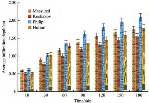
The values of performance indices such as RMSE, ME and MPD for the three infiltration models (Kostikov’s, Philip’s and Horton’s) showed realistic fits (Table 6). All the models have good capabilities for prediction of cumulative infiltration depth at the selected points. The RMSE values were found in the range of 0.073 cm to 0.341 cm, 0.041 cm to 1.261 cm and 0.059 cm to 0.153 cm for Kostikov’s, Philip’s and Horton’s infiltration models, respectively for all the six points whereas the average values of RSME were calculated as 0.185 cm for Kostikov’s, 0.235 cm for Philip’s and 0.096 cm for Horton’s models. The values of RMSE were found in close agreement as reported by Duan et al.[54] Similarly, Patle et al.[17] found RMSE values in the range of 0.09 to 7.02 with an average value of 2.07 and reported that the model can successfully be used for prediction of infiltration rate. The ME values were observed from 38% to 98 % for Kostikov’s, and 80% to 97% for Horton’s model. The ME at Point 5 for Philip’s model did not give meaningful values because prediction at that Point 5 was not good. However, values of ME for Horton’s model were found to be in the acceptable range[55]. MPD values also showed the satisfactory prediction by the infiltration models for all the selected points. Similarly, the comparison between observed and predicted infiltration depths for three tested models further verified the prediction capability of these infiltration models (Figure 4). Hsu et al.[56] evaluated three models (Green-Ampt, Philip and Horton) and demonstrated that all three models provided similar fits to the numerical results in terms of infiltration rates.
The Horton’s model provided the lowest mean values for RMSE, highest mean values for ME, lowest mean values for MPD. Infiltration can be well-described by the Horton’s model at the selected site. Al-Azawi[57] evaluated the six infiltration models on relatively course-textured and homogenous soil and reported that Horton’s model performance was most realistic. Kostikov’s gave a very good representation of infiltration when compared with the Philip’s model. Berndtsson[58] compared two commonly used infiltration model on heavy calcareous clay soils and found that the Horton’s model performed slightly better than the Philip’s model. Similarly, Hsu et al.[56] concluded that Horton’s model differed most as compared to the other two models. These results also agreed with the finding of Ogbe et al.[2] who ranked Horton’s model in the 1st, Kostikov’s model in the 2nd and Philip’s in the 3rd positions. Overall analysis based on the other research studies indicated that findings of the present study were satisfactory, and Horton’s model can be used to predict the infiltration depth at the study area most precisely.
Table 6 Values of performance indices between the predicted and measured cumulative infiltration
Points
Kostikove’s Model
Z = ntk Philip’s Model Z = St0.5 + At ZHorton’s Model = (fo-fc)e-kt + fc RMSE
/cm ME
/% MPD RMSE
/cm ME
/% MPD RMSE
/cm ME
/% MPD Point-1 0.341 38 –3.543 0.041 99 0.024 0.085 96 0.209 Point-2 0.221 76 –2.153 0.070 98 0.617 0.100 95 0.099 Point-3 0.196 63 –2.412 0.095 91 0.884 0.059 97 0.054 Point-4 0.331 33 –3.791 0.113 92 –0.092 0.145 87 –0.023 Point-5 0.129 86 –1.718 1.261 –1255 5.789 0.153 80 –0.158 Point-6 0.073 98 0.920 0.049 99 0.367 0.100 96 0.130 Mean* 0.185 78 –1.992 0.235 64 2.140 0.096 94 0.127 Note: *Mean values calculated based on the average of six points as given in Tables 3, 4 and 5.
Figure 4 Comparison between predicted and measured average cumulative infiltration
4 Conclusions
Based on the evaluation of three infiltration models, all the models showed good agreement with the measured cumulative infiltration depths in the field using the estimated model’s parameters. The acceptable ranges of model performance indicators such as RMSE, ME and MPD indicated that the evaluated infiltration models realistically simulate cumulative infiltration depth under the field conditions of the study area. The accurate prediction of cumulative infiltration depth using these infiltration models’ parameters showed that models’ parameters must be modified in local soil conditions. It was also analyzed that Horton’s model gave a better fit to the measured cumulative infiltration depth than the Kostikov’s and Philip’s models. Horton’s model provided the best simulation of infiltration data in the study area as Horton’s Model showed highest value ME (94%) and the lowest value of MPD (0.127). Application of these infiltration models under verified field conditions leads to simulate the cumulative infiltration depth. It should also help to adjust stream discharge, slope, and field geometry according to the varying field infiltration rate, especially during the surface irrigation.
Acknowledgements
Authors are grateful to Department of Agricultural Engineering Bahauddin Zakariya University, Multan for allowing them to use their facilities.
[References]
[1] Musa J J, Adeoye P A. Adaptability of infiltration equations to the soils of the Permanent Site Farm of the Federal University of Technology, Minna, in the Guinea Savannah Zone of Nigeria. Au. Journal of Technology, 2010; 14(2): 147–155.
[2] Ogbe V B, Jayeoba O J, Ode S O. Comparison of four soil infiltration models on a sandy soil in Lafia, Southern Guinea Savanna Zone of Nigeria. Production Agriculture and Technology, 2011; 7(2): 116–126.
[3] Shakoor A, Arshad M, Tariq A R, Ahmad I. Evaluating the role of bentonite embedment in controlling infiltration and improve root zone water distribution in coarse soil. Pak. J. Agri. Sci., 2012; 49(3): 375–380. [4] Arshad I, Sarki A, Khan E Z A. Analysis of Water transmission behavior
in sandy loam soil under different tillage operations of m6ould board plough applying /using different infiltration models. International Journal for Research in Applied Science & Engineering Technology, 2015; 3(VII): 254–266.
[5] Daly E, Porporato A. A review of soil moisture dynamics: From rainfall infiltration to ecosystem response. Environmental Engineering Science, 2005; 22(1): 9–24.
regime and water balance in a transplanted rice field experiment with reduced irrigation. Water, 2017; 9(4): 248.
[7] Hickok R B, Osborn H B. Some limitations on estimates of infiltration as a basis for predicting watershed runoff. Transactions of the ASAE, 1969; 12(6): 0798–0800.
[8] Feki M, Ravazzani G, Ceppi A, Milleo G, Mancini M. Impact of infiltration process modeling on soil water content simulations for irrigation management. Water, 2018; 10(7): 850.
[9] Essig E T, Corradini C, Morbidelli R, Govindaraju R S. Infiltration and deep flow over sloping surfaces: Comparison of numerical and experimental results. Journal of Hydrology, 2009; 374(1-2): 30–42. [10] Haghiabi A H, Abedi-Koupai J, Heidarpour J M, Mohammadzadeh-Habili
J. A new method for estimating the parameters of Kostiakov and modified Kostiakov infiltration equations. World Applied Sciences Journal, 2011; 15(1): 129–135.
[11] Liu D D, She D L, Yu S E, Shao G C, Chen D. Predicted infiltration for sodic/saline soils from reclaimed coastal areas: Sensitivity to model parameters. The Scientific World Journal, 2014; 2014: 1–12.
[12] Rashidi M, Seyfi K. Field comparison of different infiltration models to determine the soil infiltration for border irrigation method. Am Eurasian J Agric Environ Sci., 2007; 2(6): 628–632.
[13] Walker W R, Prestwich C, Spofford T. Development of the revised USDA–NRCS intake families for surface irrigation. Agric Water Manag, 2006; 85(1-2): 157–164.
[14] Cuenca R H. Irrigation system design: an engineering approach. Prentice Hall, Englewood Cliffs, 1989.
[15] Rao M D, Raghuwanshi N S, Singh R. Development of a physically based 1D-infiltration model for irrigated soils. Agric Water Manag, 2006; 85(1-2): 165–174.
[16] Rahman G A, Talaat A M, Zawe C. Assessment of infiltration rate for sustainability of reclaimed area in Harare region Zimbabwe. Middle East Journal of Agriculture, 2016; 5(1): 1–5.
[17] Patle G T, Sikar T T, Rawat K S, Singh S K. Estimation of infiltration rate from soil properties using regression model for cultivated land. Geology, Ecology, and Landscapes, 2019; 3(1), 1–13.
[18] Mishra S K, Tyagi J V, Singh V P. Comparison of infiltration models. Hydrol Process, 2003; 17(13): 2629–2652.
[19] Oku E, Aiyelari A. Predictability of Philip and Kostiakov infiltration model under inceptisols in the Humid Forest Zone, Nigeria. Kasetsart Journal: Natural Science, 2011; 45: 594–602.
[20] Xing X, Li Y, Ma X. Effects on infiltration and evaporation when adding rapeseed-oil residue or wheat straw to a loam soil. Water, 2017; 9(9): 700.
[21] Green W H, Ampt G A. Studies on soil physics: I. Flow of air and water through soils. J Agric Sci, 1911; 4: 1–24.
[22] Williams J R, Ouyang Y, Chen J S, Ravi V. Estimation of infiltration rate in the vadose zone: application of selected mathematical models, vol II. USEPA EPA/600/R-97/128a, 1998.
[23] Gundalia M. Estimation of infiltration rate based on complementary error function peak for Ozat watershed in Gujarat (India). International Journal of Hydrology, 2018; 2(3): 289‒294.
[24] Ravi V, Williams J R. Estimation of infiltration rate in the vadose zone: Compilation of simple mathematical models. Vol. I, USEPA EPA/600/R-97/128a, 1998.
[25] Haghighi F, Gorji M, Shorafa M, Sarmadian F, Mohammadi M H. Evaluation of some infiltration models and hydraulic parameters. Spanish Journal of Agricultural Research, 2010; 8: 210–217.
[26] Fashi F H, Sharifi F, Kamali K. Modelling infiltration and geostatistical analysis of spatial variability of sorptivity and transmissivity in a flood spreading area. Spanish Journal of Agricultural Research, 2014; 12(1): 277–288.
[27] Igbadun H E, Idris U D. Performance evaluation of infiltration models in a hydromorphic soil. Nig. J. Soil & Env. Res, 2007; 7: 53–59.
[28] Adindu R U, Igbokwe K K, Dike I I. Philip model capability to estimate infiltration for soils of Aba, Abia State. Journal of Earth Sciences and Geotechnical Engineering, 2015; 5(2): 63–68.
[29] Roohian M H, Miring U A, Saghafian B, Delafkar H. Horton’s infiltration model calibration in Nimrod watershed, Firoozkooh, Tehran Province, 3rd Erosion & Sediment National Conference, Tehran, 2005.
[30] Mbagwu J S C. Quasi-steady infiltration rates of highly permeable tropical moist savannah soils in relation to land use and pore size
distribution. Soil Technology, 1997; 11: 185–195.
[31] Allison L E, Moodie C D. Carbonate. In: Methods of soil analysis (Black C A, Ed). Part 2. Agron.Monogr. Am. Soc. Agron., Madison, WI. 1965; pp.1379–1396.
[32] Gee G W, Bauder J W. Particle size analysis. In: Methods of soil analysis (Klute A, Ed), Part 1, 2nd Ed. Agronomy No. 9, Am. Soc. Agron., Madison, WI. 1986; pp.825–844.
[33] Davies D B, Finney J B, Richardson S J. Relative effects of tractor weight and wheel-slip in causing soil compaction. J Soil Sci, 1973; 24: 399–409.
[34] Klute A, Dirksen C. Hydraulic conductivity and diffusivity. In: Methods of soil analysis (Klute A, Ed). Part 1. Physical and mineralogical methods, 2nd ed. Agronomy monographs, Madison, WI, 1986; pp.687–734.
[35] Kostiakov A N. On the Dynamics of the coefficient of water percolation in soils and the necessity of studying it from the dynamic point of view for the purposes of Amelioration. Trans. 6th Comm. Int. Soil Science Society, Moscow, Part A, 1932: 17. (in Japanese)
[36] Philip J R. The theory of infiltration: 4. Sorptivity and algebraic infiltration equations. Soil Science, 1957; 84: 257–264.
[37] Horton R E. An approach towards a physical infiltration capacity. Soil Science Society of America Proceedings, 1940; 5: 399–417.
[38] Uloma A R, Samuel A C, Kingsley I K. Estimation of Kostiakov’s infiltration model parameters of some sandy loam soils of Ikwuano– Umuahia, Nigeria. Open Transactions on Geosciences, 2014; 1(1): 34–38.
[39] Jaynes R A, Gifford G F. An in-depth examination of the Philip equation for cataloging infiltration characteristics in rangeland environments. Journal of Range Management, 1981; 34(4): 285–295.
[40] Machiwal D, Jha M K, Mal B C. Modelling infiltration and quantifying spatial soil variability in a wasteland of Kharagpur, India. Biosystems Engineering, 2006; 95(4): 569–582.
[41] Turner E R. Comparison of infiltration equations and their field validation with rainfall simulation. Maryland: University of Maryland, 2006.
[42] Haghighi F, Gorji M, Shorafa M, Sarmadian F, Mohammadi M. Evaluation of some infiltration models and hydraulic parameters. Spanish Journal of Agricultural Research, 2010; 8(1): 210–217.
[43] Mudiare O J, Adewumi J K. Estimation of infiltration from field-measured sorptivity values. Nigeria Journal of Soil Research, 2000; 1: 1–3.
[44] Nash J E, Sutcliffe J V. River flow forecasting through conceptual models. Part 1-A: Discussion of principles. J. Hydrol. (Amsterdam), 1970; 10: 282–290.
[45] Fang Q, Ma L, Yu Q, Malone R W, Saseendran S A. Ahuja L R. Modeling nitrogen and water management effects in a wheat-maize double-cropping system. Journal of Environmental Quality, 2008; 37: 2232–2242. [46] Bakhsh A, Bashir I, Farid H U, Wajid S A. Using CERES-wheat model
to simulate grain yield production function for Faisalabad, Pakistan, Conditions. Expl Agric., 2013; 49(3): 461–475.
[47] Farid H U, Bakhsh A, Mahmood-Khan Z, Ahmad N, Ahmad A. Using CERES-Wheat model for simulating fertilizer application rates to maximize grain yield. Journal of Agricultural Sciences, 2015; 7(7): 115–127.
[48] Kargas G, Chatzigiakoumis I, Kollias A, Spiliotis D, Massas I, Kerkides P. Soil salinity assessment using saturated paste and mass soil: Water 1:1 and 1:5 ratios extracts. Water, 2018; 10 (11): 1589.
[49] Ganjegunte G K, Clark J A, Parajulee M N, Enciso J, Kumar S. Salinity management in pima cotton fields using sulfur burner. Agrosystems, Geosciences & Environment, 2018; 1: 180006.
[50] Blair A W, Reddell D L. Evaluation of empirical infiltration equation for blocked furrow infiltrometer. Chicago, ASAE Winter Meeting, 1983; pp.83–2521.
[51] Serralheiro R P. A study of furrow irrigation on a Luvisoil. Evora: University of Evora, 1988.
[52] Leão T P, Perfect E. Modeling water movement in horizontal columns using fractal theory. Brazilian Journal of Soil Science, 2010; 34: 1463–1468. (in
Portuguese)
3(6): 1–7.
[54] Duan R, Fedler C B, Borrell J. Field evaluation of infiltration models in lawn soils. Irrigation Science, 2011; 29: 379–389.
[55] Alkassem Alosman M, Ruy S, Buis S, Lecharpentier P, Bader J C, Charron F, et al. An improved method to estimate soil hydrodynamic and hydraulic roughness parameters by using easily measurable data during flood irrigation experiments and inverse modelling. Water, 2018; 10(11): 1581.
[56] Hsu S M, Ni C F, Hung P F. Assessment of three infiltration formulas based on model fitting on Richards equation. Journal of hydrologic Engineering, 2002; 7(5): 373–379.
[57] Al-Azawi S A. Experimental evaluation of infiltration models. Journal of Hydrology, 1985; 24(2): 77–88.