The Thirty-Third AAAI Conference on Artificial Intelligence (AAAI-19)
Active Sampling for Open-Set Classification without Initial Annotation
Zhao-Yang Liu, Sheng-Jun Huang
∗College of Computer Science and Technology, Nanjing University of Aeronautics and Astronautics Collaborative Innovation Center of Novel Software Technology and Industrialization
Nanjing 211106, China {zhaoyangliu, huangsj}@nuaa.edu.cn
Abstract
Open-set classification is a common problem in many real world tasks, where data is collected for known classes, and some novel classes occur at the test stage. In this paper, we focus on a more challenging case where the data examples collected for known classes are all unlabeled. Due to the high cost of label annotation, it is rather important to train a model with least labeled data for both accurate classifica-tion on known classes and effective detecclassifica-tion of novel classes. Firstly, we propose an active learning method by incorporat-ing structured sparsity with diversity to select representative examples for annotation. Then a latent low-rank representa-tion is employed to simultaneously perform classificarepresenta-tion and novel class detection. Also, the method along with a fast opti-mization solution is extended to a multi-stage scenario, where classes occur and disappear in batches at each stage. Exper-imental results on multiple datasets validate the superiority of the proposed method with regard to different performance measures.
Introduction
In traditional supervised learning tasks, it is commonly as-sumed that the class labels are identical in the training phase and test phase. However, in many real applications, the la-bel set expands as more novel classes occur during the test phase. For example, in face recognition problem, the model is trained with data collected for a prefixed set of people, and then is applied to real environment with many new persons (Zhang and Patel 2017); in automated genre identification of web pages, web page genres evolve, and the predefined genre palette may not cover all the genres existing in a large corpus during the test phase (Guru et al. 2016).
Such problems are formalized as a learning framework called open-set classification (Scheirer et al. 2013). In this framework, training examples are all collected from known classes, while test examples are from both the known classes and some other novel classes. The target of open-set classi-fication is to train a model that on one hand can accurately classify examples of known classes, and on the other hand
∗
This work was supported by National Key R&D Pro-gram of China (2018YFB1004300), NSFC (61503182, 61876081, 61732006).
Copyright c2019, Association for the Advancement of Artificial Intelligence (www.aaai.org). All rights reserved.
can successfully detect those from novel classes. Obviously, this is a much more challenging task than close-set classifi-cation.
There are some studies trying to solve this problem in different ways. For example, (Yu et al. 2017; J´unior et al. 2016) detects novel data by the distance difference be-tween known data and novel class data, (Masud et al. 2010; Guru et al. 2016) uses clustering to filter novel class data. Most of these methods require a large set of annotated ex-amples from known classes to train the classification model, which however, is usually unavailable in real cases. Actu-ally, in real tasks, label annotation is usually expensive and time costly. Thus a more practical scenario is that we have a dataset collected from known classes, but all examples are unlabeled. For example, face images may automatically col-lected by detecting faces from a video of a known set of people, but not precisely annotated with person ID; and web pages of predefined genre set may be collected in batch by a spider, yet it is not annotated for each page. This situa-tion leads to a more challenging task of learning with least labeled data.
Active learning is a primary approach for learning from limited labeled data with high annotation cost. It actively se-lect the most important examples to query their labels, and try to train an effective model with least labeled data. In this paper, we propose an Active Sampling algorithm for Open-set Classification without Initial Annotation, and ASOCIA for short. Specifically, given no initial labeled data, it is not applicable to select the most important instances based on the model prediction. Instead, active sampling of represen-tative examples with no need of label information is a better choice.
phase, we introduce a fast solution based on incremental SVD (Berry, Dumais, and O’Brien 1995). We also extend the method to a more dynamic environment with multiple test stages, and at each stage some novel classes occur while some known classes disappear.
Experiments are performed on multiple datasets to vali-date the effectiveness of the proposed method on open-set classification. Results with regard to accuracy and F-1 mea-sure show that our method achieves better performance on both the classification of known classes and detection of novel classes.
Our main contributions are summarized as follows: • The ASOCIA framework is proposed for a novel and
chal-lenging setting of open-set classification without initial annotation.
• A new strategy incorporating structure sparsity and diver-sity is proposed for active selection of representative ex-amples. Also, the discriminative low-rank representation with a fast solution is introduced for classifying known classes and detecting novel classes.
• Experimental study is performed to validate the effective-ness of the proposed method on both the active sampling and model performance.
The rest of the paper is organized as follows. In the next section, related studies from different aspects are summa-rized and discussed. Then we propose the ASOCIA frame-work with detailed introduction on active sampling and low-rank representation learning. After that, experimental results are presented, followed by the conclusion.
Related work
Open-Set Classfication
Semi-supervised methods make use of both the labeled data and unlabeled test data which contain novel class data to train the model. In LACU (Da, Yu, and Zhou 2014), the augment risk is introduced to adjust the separator closer to the labeled region. While in (Guru et al. 2016; Masud et al. 2010), clustering technique is used to construct the boundary for filtering examples of novel class.
Open-set classification has attracted many research inter-ests. In (Scheirer et al. 2013), a open risk is introduced into the supervised classification model. After that, probability models (Scheirer, Jain, and Boult 2014; Zhang and Patel 2017) are proposed based on the open risk concept. The EVT approach (Scheirer et al. 2011) is adopted to split the score list of test data and divide them into novel or known data. The methods in (J´unior et al. 2016) and (Bouguelia, Belaid, and Belaid 2014) detect novel class by the distance of test data to labeled training data. In (Yu et al. 2017), authors adopt adversarial learning to generate pseudo negative data which are close to each known class.
Outlier detection techniques are also used for open-set classification by treating the examples from novel classes as outliers. The method in (Mu, Ting, and Zhou 2017) uses iForest (Liu, Ting, and Zhou 2008) to detect anomaly data which contain novel class data. The method in (Mu et al. 2017) uses matrix sketch technique to store main
known class information and compute inner products be-tween sketch matrix rows and test data to recognize novel class. Due to the use of matrix sketch technique, this method may need lots of labeled data.
In addition, other problems such as zero-shot learning (Xian et al. 2016), the attribute-incremental learning (Vap-nik, Vashist, and Pavlovitch 2009), the class incremental learning (Kuzborskij, Orabona, and Caputo 2013) are also related to the open-set classification problem. While most methods mentioned above utilize many labeled data with-out considering limited annotation cost, and in real world, a new item often starts with data collection and annotation, no plenty of data available.
Active Learning
Active learning is a primary approach to deal with limited labeled data. It selects the most important examples to query their labels from the oracle. Different criteria have been pro-posed to estimate how important an example is for improv-ing the classification model (Huang, Jin, and Zhou 2010; Huang and Zhou 2013).
In our problem setting, we need to select a batch of exam-ples from the unlabeled dataset for once. And experimental design methods fit the data selection situation. In (Yu, Bi and Tresp 2006), authors propose the TED method for transduc-tive experimental design, which tends to select data repre-sentative to those yet unexplored data. Based on the idea of data construction, (Yu et al. 2008; Shi and Shen 2016) trans-forms the TED as a convex problem and can get a global optimal solution. Another method ANLR (Hu et al. 2013) further improves the result by local reconstruction with only neighbors. (Nie et al. 2013) proposes the RRSS where the
L2,1norm is adopted to constrain the data construction loss
and the relationship matrix of training data.
Low-Rank Representation
In many studies (Narayanan and Mitter 2010; Donoho and Grimes 2003), a common assumption is that high-dimensional data lies in a low-high-dimensional subspace and it is reasonable in reality to structural data such as images, texts and digital audio files. So the data could be compressed from high dimension to low dimension. LRR (Liu, Lin, and Yu 2010) can be seen as a compressed sensing technique, which tries to minimize the rank of the relationship matrix. (Liu, Lin, and Yu 2010) solves the problem with a strong as-sumptions that the training data of each class are sufficient and the noises of data are at low level. (Liu and Yan 2011) ease the problem by introducing the effects of hidden data.
The ASOCIA Framework
Problem Formulation
In traditional supervised learning, model is trained on a la-beled set{(xi, yi)}n
i=1 withnexamples, where yi ∈ Y is
the class label of thei-th instance, andY ={1,2,· · · , K} is the close-set of K class labels. At the test phase, each in-stance belongs to one of theKclasses inY. The task is to learn a modelf(x) : X →Y to classify test instances into one of theKclasses.
In a classical open-set classification task, the training data X = {(xi, yi)}ni=1 consists of n examples from K
known classesY ={1,2,· · ·, K}. While in the test phase, the test set consists of instances from the open-set classes
Y = {1,2,· · · , K, K + 1,· · ·, K +M}, where the M
novel classes K + 1,· · ·, K +M are unseen during the training phase. The task is to learn a modelf(x) : X → {1,2,· · ·, K, novel}, where thenovelrepresents all novel classes.
In this paper, we consider a special case of open-set clas-sification with no initial annotation. At the beginning of the training phase, we are given a dataset X = {xi}ni=1
with n instances. Each instance belongs to one of the K
classes in Y = {1,2,· · · , K}. However, the ground-truth annotation yi is not available for all instances xi ∈ X.
We need to actively sample a batch of important instances from X, query their class labels, and then train a model
f(x) :X → {1,2,· · ·, K, novel}to perform classification of known classes as well as detection ofnovelclasses.
Active Selection of Representative Examples
In the ASOCIA framework, we have no initially labeled data even for the known classes, and need to actively se-lect a batch of most important examples from the unla-beled pool to annotate. Without a classification model to estimate the uncertainty or informativeness of an unla-beled instance, it is more practical to perform active sam-pling based on representativeness. Among the active learn-ing methods, experimental design (Yu, Bi, and Tresp 2006; Nie et al. 2013) has shown effective performance for repre-sentative sampling.In (Yu, Bi, and Tresp 2006), a transductive experimental design (TED) method is proposed to select the examples that can best represent the whole data using a linear represen-tation. Formally, given a datasetX = [x1,x2,· · · ,xn] ∈ Rd×n with n instances of d-dimensional feature vectors,
TED tries to select a setBofmexamples fromX with the following objective function.
min
B,W n X
i=1
kxi−Bwik22+γkwik22
(1)
s.t. B ⊂X,|B|=m, W = [w1,· · ·,wn]∈Rm×n.
Herewi is the linear weight vector reflecting the relations
between the selected examples and the instancexi.
The problem in Eq. 1 is NP-hard, and is solved with greed optimization (Yu, Bi, and Tresp 2006). Later, a more robust method is proposed in (Nie et al. 2013) by introducing struc-tured sparsity. Specifically, this method dose not directly se-lect a subset B fromX. Instead, all examples are used to
represent each instance xi with the weight vectorwi of n
dimensions. The objective functions is as follows.
min
W k(X−XW) >k
2,1+γkWk2,1, (2)
where the second term with`2,1-norm onW aims to achieve
structured sparsity. On one hand, the loss function will be less sensitive to outliers compared to that in Eq. 1; and on the other hand, the`2,1-norm leads to a row-sparse solution
ofW. After the optimization of the above problem, the rep-resentative examples are selected according to the row-sum values of absoluteW. A larger sum value of|wi|implies
thatxicontributes more to represent other examples, thus is
more representative and should be selected to annotate. When we sort the examples by the row-sum values of the absoluteW, there could be some similar examples among the top ranked examples, which may contain redundant in-formation. Annotating such redundant examples will con-tribute less to the model training, and thus leads to waste of annotation cost. To solve this problem, we propose to incor-porate diversity into the objective function when optimizing the weight vectors. Specifically, we have:
min
W k X−XW
>
k2,1+γkWk2,1+λkW W>k2F, (3)
whereγandλare two trade-off parameters. The third term minimizes the correlations among different rows ofW, and thus is expected to enhance the diversity of selected exam-ples. In summary, the objective of Eq. 3 is to select examples that can well represent the whole dataset via linear combi-nation, have structured sparsity and high diversity. Such se-lected examples are expected to be most helpful to train an effective model.
Next we will discuss the optimization of Eq. 3. We adopt an approach similar in (Nie et al. 2013) to solve this convex problem. By setting the derivative of Eq. 3 to zero, we have:
X>XW U−X>XU+γV W+ 4λW W>W = 0. (4)
BothUandV are diagonal matrix, whose elements are com-puted according to (Nie et al. 2010):
Ui,i= 1
kxi−Xwik
; Vi,i= 1
kwik.
wherewiandwirepresenti-th column andi-th row
respec-tively. By further denotingM =W W>, after calculatedU
andV, fixM =W WT, then we can updateW andM al-ternately, repeat the procedure until convergence condition satisfied.
The algorithm for active sampling is summarized in Al-gorithm 1. Note in the experiments of multiple test phases, we also use this algorithm to select additional examples for annotation at each stage.
Low-Rank Representation Learning
Algorithm 1Active Sampling
Input: The dataX∈Rd×n; parametersγandλ
Output: The selectedmrepresentative examples;
1: InitializeW ∈Rn×n, andU, V as diagonal matrices;
2: repeat
3: Calculate diagonal elements:Ui,i= kxi−X1 wik; 4: Calculate diagonal elements:Vi,i=kw1ik ;
5: CalculateM =W W>;
6: fori= 1tondo
7: Calculate each column ofW as
8: wi=Ui,i Ui,iX>X+γV + 4λM
−1
X>xi; 9: UpdateM byM =W W>;
10: end for
11: until(satisfy the convergence condition)
12: Calculate the row-sum values of|W|;
13: Return themexamples with largest row-sum values.
learning has achieved great success in various applications (Liu and Yan 2011; Zhou, Lin, and Zhang 2016). The basic assumption of LRR is that data from the same class should be distributed in the same low-dimensional subspace. While the dimension of the subspace corresponds to the rank of the representation matrix, LRR tries to find the lowest-rank rep-resentation that can represent the data examples with linear combinations of given dictionary.
Given the data matrixX∈Rd×n, the original LRR
min-imizes the following objective:
min
Z Rank(Z) s.t. X=AZ, (5)
whereAis the dictionary. To efficiently solve this problem, some alternative approaches with nuclear norm are proposed (Cai, Candes, and Shen 2010).
In our setting, very limited labeled data is available, and thus favors the methods that are more robust and require less examples. Latent LRR (Liu and Yan 2011) is a representa-tive approach applicable to less data. It tries to exploit hid-den data, and decomposes the data matrixXinto two parts: a low-rank partXZ for principle features and a low-rank partLXfor salient features, as formalized in the following equation.
min
Z,LkZk∗+kLk∗ (6)
s.t. X =AZ+LX.
The Algorithm
After solving the optimization problem in Eq. 6, the matrix
Z captures the affiliation between data examples. Figure 1 visualizes the affiliation matrix of ExtendedYaleB dataset with 6 known classes. It can be observed that data from the same class have strong correlations. This affiliation matrix thus could be utilized for classification as well as novel class detection. Specifically, denote byXl∈Rd×nthe set of
rep-resentative examples selected via active sampling, and we have known their labels yl. The corresponding affiliation
matrix is denoted by Zl. In the test phase, a new instance
Figure 1: Visualization of the affiliation matrix Z with 6 known classes on ExtendedYaleB dataset
0.010 0.015 0.020 0.025 0.030 0.035 class mass value
0 200 400 600 800 1000
number
known_data new_data
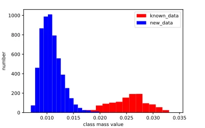
Figure 2: true score(class mass value) distribution of test data
xo from open set is to be classified into one of the known
classes or a novel class. If we add a test instancexointoXl,
then we can have a new affiliation matrix (Zhang, Lin, and Zhang 2013):
ˆ
Z∗= ˆVSˆVˆ>,
where Sˆ is a block diagonal matrix and Vˆ> comes from
SV D(Xl+o) = ˆUΣ ˆˆV>,Zˆ∗has one more row and one more
column thanZl. We then delete the last column, and denote byzothe absolute value of the last row ofZˆ∗.zodescribes
how the test example xo is affiliated with the labeled data Xl. Then we calculate the score for each of the K known classes as:
Cok = Pm
i=1I(yl(i) =k)·zo(i)
Pm
i=1I(yi=k)
, (7)
whereI(·)is the identity function.Ck
o estimates how likely
xobelongs to classk.
Next, we need to decide whether xo belongs to a novel
class or not. Inspired by (Prewitt, Judith, and L. Mendel-sohn 1966) which is prevalent in picture precessing, we use a iterative method to determine the threshold for distinguish known and novel classes. Given an instancexoof the test set Xt, we firstly calculate the scoreso = arg maxk=1:KCok,
smin among all test data. After that the threshold is tem-porally set as(smax+smin/2), and the test set is divided into two subsets according to the threshold. Then we update
smax andsmin by the mean scores of the two subsets, re-spectively. And the threshold updates as(smax+smin/2).
This process will be repeated until the threshold value con-verges to a stable value. Figure 2 shows an example of the score distribution over the test data on ExtendedYaleB. It demonstrate that the above method can find a accurate threshold for separating known and novel classes. At last, if the test instancexois identified as from known classes, then
its class label will be further determined asarg maxkCok.
Although some efficient solutions have been proposed for the problem in Eq. 6 (Zhang, Lin, and Zhang 2013; Liu and Yan 2011), it is still can not get the solution directly because we do not know the value ofSl; moreover, it is not
scalable because we need to compute the affiliation matrix for each test example during the test phase. To overcome this problem, we adopt the incremental SVD (Berry, Dumais, and O’Brien 1995) to obtain a fast solution for calculating the affiliation matrix. Assume that we have the initial af-filiation matrix of training dataZl = VlSlVl> forXl, and SVD(Xl) =UlΣlVl>. We add test data matrixXt∈Rd×m
toXl to form the new data matrix Xnew = [Xl;Xt]. We can make use of the SVD results overXlinstead of perform SVD from scratch on Xnew. With the result from (Berry, Dumais, and O’Brien 1995), we have:
SVD(Xnew) =UnewΣnewVnew> =UlΣl[Vl>;V > t ],
whereVt= Xt>UlΣ−l1. Thus for the case of adding a new test instancexo, we can have:
ˆ
Z∗= ˆV SlVˆ>,
andVˆ> =
Vl>;Vt>[:, o]
. It can be further written as:
ˆ
Z∗= ˆV(Vl>ZlVl) ˆV>.
With this incremental solution to calculate the affiliation matrix, we can finally get efficient method to perform clas-sification and novel class detection. The whole procedure of our method is summarized in Algorithm 2.
Experiments
Datasets and algorithms
In our experiments, three datasets are used to examine the performance of the compared methods. ExtendedYaleB (Lee, Ho, and Kriegman 2005) has 28 classes, each of which has 576 images. Each image is resized to48×42. Fashion-MNIST (Xiao, Rasul, and Vollgraf 2017) consists of 70000 examples from 10 classes, where each example is a28×28grayscale image of clothes or shoes. We sample 500 instances for each class from those two datasets. Coil20 (S.A.Nene, Nayar, and H.Murase 1996) contains 20 classes, each of which has 72 examples.
The following methods are compared with our proposed method. OneClass SVM (Sch¨olkopf et al. 2001) is a base-line to learn a model for the known classes, and then can be applied to detect novel classes. MOC-SVM incorporates the
Algorithm 2The ASOCIA Algorithm
Input: Unlabeled datasetX ∈Rd×n; InitializeA∈Rn×n;
1: Perform Algorithm1 onX to select the representative examplesXl;
2: Learn the low-rank representationZlofXl;
3: ClearZlby setting non-block diagonal area to zero 4: Perform SVD overXl: SVD(Xl) =UlΣlVl> 5: Incremental SVD over test dataXt:Vt=Xt>UlΣ−
1
l 6: Compute the affiliation matrixZi∗for each example
7: Compute the scoresifor each example
8: Compute the threshold:τ 9: foreachxi∈Xtdo
10: ifsi< τ then
11: xiis detected as from novel class 12: else
13: xiis classified asyi=argmaxkCik
14: end if
15: end for
one-vs-rest strategy with OneClass SVM to perform open-set classification. SENC (Mu et al. 2017) uses matrix sketch techniques to store data information and distinguish new data and classify known class data by the sketch matrix. ASG (Yu et al. 2017) adopts adversarial learning to find a boundary around seen class data, and achieved state-of-the-art performance for open-set classification. ASOCIA-0 is a baseline of our method that simply ignore the diversity dur-ing active selection, i.e., it setsλ= 0in Eq. 3.
Result on the open-set classification
For each dataset, we set 20% of the class labels as known, and others as novel classes. For ExtendedYaleB, half of the 5 known classes are randomly selected as the training set, from which the ASOCIA algorithm will actively select 150 examples from each class for annotation. At test stage, the other half of training examples from known classes together with all examples from unknown classes are used as the test set. Similar data partition is applied to Fashion-MNIST and Coil20, which have 2 and 4 known classes, respectively. The data partition is repeated for 10 times, and the average re-sults are reported.
Because of the imbalanced size between known data and novel data, the measurements used here are accuracies of known class and novel class respectively: Accuracy−
known = Mknown
Nknown, where Mknown is the number of
known data that are classified correctly to the true class, and
Nknownis the number of true known data in test data.
Sim-ilarly, for novel class data, Accuracy−novel = Mnovel
Nnovel.
Besides, we also adopt F1-measure to evaluate the over-all performance on over-all test data (Yu et al. 2017; Mu et al. 2017). The results are showed in Table 1, 2 and 3, respec-tively. OneClass SVM can only distinguish between known and novel classes; and thus noaccuracy-knownandF1-total available for this method.
Table 1: Open-set classification result of ExtendedYaleB: Best results are bold, OC could not classify known data with detail label, so some results are NA.
Method OC MOC SENC ASG ASOCIA-0 ASOCIA
Accuracy-known NA 0.515±0.034 0.240±0.029 0.876±0.023 0.935±0.018 0.939±0.016
Accuracy-novel 0.404±0.027 0.663±0.064 0.528±0.008 0.898±0.036 0.999±0.002 0.999±0.001
F1-total NA 0.340±0.052 0.140±0.032 0.838±0.003 0.964±0.008 0.966±0.009
Table 2: Open-set classification result of Coil20: Best results are bold, OC could not classify known data with detail label, so some results are NA.
Method OC MOC SENC ASG ASOCIA-0 ASOCIA
Accuracy-known NA 0.751±0.049 0.443±0.013 0.896±0.085 0.958±0.026 0.980±0.018
Accuracy-novel 0.591±0.012 0.950±0.014 0.377±0.015 0.904±0.034 0.970±0.038 0.996±0.003
F1-total NA 0.770±0.036 0.225±0.007 0.788±0.069 0.927±0.059 0.982±0.009
Table 3: Open-set classification result of Fashion-MNIST: Best results are bold, OC could not classify known data with detail label, so some results are NA.
Method OC MOC SENC ASG ASOCIA-0 ASOCIA
Accuracy-known NA 0.760±0.057 0.345±0.093 0.824±0.043 0.818±0.128 0.810±0.031 Accuracy-novel 0.196±0.010 0.574±0.042 0.574±0.026 0.178±0.060 0.674±0.162 0.720±0.160
F1-total NA 0.439±0.030 0.225±0.055 0.322±0.017 0.539±0.077 0.571±0.092
Table 4: Performance on multiple test stages of ExtendedYaleB: Best results are bold, OC could not classify known data with detail label, so some results are NA.
Method
Stage one Stage two Stage three
Precision Recall F1-Measure Precision Recall F1-Measure Precision Recall F1-Measure
OC NA 0.599±0.046 NA NA 0.661±0.061 NA NA 0.406±0.046 NA MOC 0.605±0.047 0.938±0.042 0.725±0.048 0.640±0.037 0.899±0.079 0.736±0.041 0.354±0.058 0.692±0.111 0.426±0.071 SENC 0.398±0.035 0.677±0.016 0.461±0.031 0.437±0.045 0.557±0.011 0.464±0.038 0.267±0.096 0.612±0.032 0.317±0.099 ActMiner 0.578±0.037 0.958±0.015 0.720±0.0.026 0.383±0.043 0.628±0.108 0.476±0.063 0.529±0.037 0.831±0.061 0.646±0.041 ASG 0.956±0.016 0.948±0.019 0.952±0.011 0.981±0.019 0.926±0.026 0.945±0.013 0.996±0.006 0.865±0.030 0.926±0.016 ASOCIA-0 0.937±0.101 0.969±0.023 0.949±0.060 0.975±0.025 0.997±0.010 0.985±0.012 0.996±0.003 0.942±0.019 0.968±0.010 ASOCIA 0.973±0.024 0.956±0.015 0.964±0.015 0.999±0.001 0.968±0.017 0.984±0.009 0.986±0.016 0.944±0.017 0.964±0.014
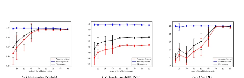
20 30 40 50 60 70 80 90 scale of the affiliation matrix 0.2
0.4 0.6 0.8 1.0
Accuracy-known Accuracy-novel F1-measure
(a) ExtendedYaleB
20 30 40 50 60 70 80 90 scale of the affiliation matrix 0.3
0.4 0.5 0.6 0.7 0.8 0.9 1.0
Accuracy-known Accuracy-novel F1-measure
(b) Fashion-MNIST
20 30 40 50 60 70 80 90 scale of the affiliation matrix 0.0
0.2 0.4 0.6 0.8 1.0
Accuracy-known Accuracy-novel F1-measure
(c) Coil20
classes and detection accuracy on novel classes. Especially, the superiority of ASOCIA over ASOCIA-0 validates that considering the diversity is helpful for active sampling of representative examples. Among the compared methods, ASOCIA-0 tends to be effective in most cases, probably benefits from the low-rank representation learning. ASG also achieves descent performance on some datasets, but is less effective on the others. One possible reason is that ASG need to identify the boundary for generating examples. While on some small datasets with limited labeled data, e.g., Coil20, it may lose its edge due to the less accurate bound-ary. In addition, ASG generates data around each known class based on the distance. So if data from different classes are close to each other, ASG may confuse to recognize the labels of data. In contrast, our model based on low-rank rep-resentation learning can distinguish data based on the sub-space where data lies in.
SENC gets relatively less effective results. In (Mu et al. 2017), the matrix sketch technique aims at large data ma-trix, and requires a large number of labeled data. While in our experiments, only a few examples are used to train the model. Besides, SENC computes inner products of the test data with every row of the sketch matrix. The datasets used here are image files. For example, for grayscale images, in-ner product of two undertint images is smaller than one un-dertint image with a dark image, so inner products of data to sketch matrix rows may not appropriate.
Result with different scales of affiliation matrix
In previous experiments, the average budget number is 30 for each class in the affiliation matrix. Here we examine how the performance changes with the increase of the affiliation matrix size. For each dataset, 6 classes are used and 3 of them are known classes and the other 3 classes are novel. The number of examples in each class is the same as previ-ous experiments. We select data from 3 known classes and the budget number is from 15 to 90. The result is showed in Figure 3.
Figure 3 shows that the method achieves a high accu-racy of novel class detection with various affiliation matrix sizes. Because in this experiment the score statistical distri-bution shows that the score range of novel data is smaller and lies in a narrow interval of unimodal distribution, so after the threshold separated the score list, novel data can always be classified correctly with high accuracy. But the score of known data is widely distributed. In the beginning, the ac-curacy of known data and the F1-measure are at low level and the standard deviation measurements are larger, After the training data grows to a certain scale, the performance stays at high level with a more steady state.
Update the model on multiple test stages
In this subsection, we examine the performance of the pro-posed method in a more challenging case with multiple test stages. In the beginning, no labeled data are available and we select 90 data from unlabeled dataset which contains 3 classes, then in every test stage, test dataset contains 6 classes, i.e., 3 novel classes are added. In each stage, we
label the selected data and merge them with labeled data se-lected previously for the model training. We set three stages until 9 classes are included in the model. Due to the equal number of known data and novel data in test dataset, we use Precision, Recall and F1-measure as measurements where known data classified correctly are seen as true positive data, novel data classified correctly are seen as true negative data. The result is showed in Table 4. ASOCIA and ASOCIA-0 have the best classification results and new data detec-tion effects. ActMiner (Masud et al. 2010) uses clustering to control the boundary which is a hypersphere determined by the furthest point to the corresponding cluster center, so it is more sensitive to outliers and may not filter new class data accurately.
Conclusion
We study a challenging case of open-set classification, where the training data is collected from known class but fully unlabeled, while the test data is from a open-set of both known and novel classes. We propose an active learn-ing approach to perform both classification of known classes and detection of novel classes. On one hand, representative sampling is incorporated with diversity to actively select the most important examples for label annotation; on the other hand, low-rank representation along with a online solution is learned to achieve discriminative features. The effectiveness of the proposed ASOCIA approach is validated on multiple datasets with regard to different performance measures. In the future, we plan to incorporate other classification tech-niques with representation learning to further improve the performance.
References
Berry, M. W.; Dumais, S. T.; and O’Brien, G. W. 1995. Us-ing linear algebra for intelligent information retrieval. Siam Review37(4):573–595.
Bouguelia, M. R.; Belaid, Y.; and Belaid, A. 2014. Effi-cient active novel class detection for data stream classifica-tion. InInternational Conference on Pattern Recognition, 2826–2831.
Cai, J.; Candes, E. J.; and Shen, Z. 2010. A singular value thresholding algorithm for matrix completion.Siam Journal on Optimization20(4):1956–1982.
Da, Q.; Yu, Y.; and Zhou, Z. 2014. Learning with augmented class by exploiting unlabeled data. In Proceedings of the 28th AAAI Conference on Artificial Intelligence, 1760–1766.
Donoho, D., and Grimes, C. 2003. Hessian eigenmaps: new locally linear embedding techniques for high-dimensional data. Technical report.
Guru, D. S.; Suhil, M.; Gowda, H. S.; and Raju, L. N. 2016. Detection of a new class in a huge corpus of text documents through semi-supervised learning. InInternational Confer-ence on Advances in Computing, Communications and In-formatics.
the 23rd International Joint Conference on Artificial Intelli-gence.
Huang, S.-J., and Zhou, Z.-H. 2013. Active query driven by uncertainty and diversity for incremental multi-label learn-ing. InProceedings of the 13th IEEE International Confer-ence on Data Mining, 1079–1084.
Huang, S.-J.; Jin, R.; and Zhou, Z.-H. 2010. Active learn-ing by querylearn-ing informative and representative examples. In Proceedings of the 23rd International Conference on Neural Information Processing Systems, 892–900.
J´unior, P. R. M.; de Souza, R. M.; de O. Werneck, R.; Stein, B. V.; Pazinato, D. V.; de Almeida, W. R.; Penatti, O. A. B.; da S. Torres, R.; and Rocha, A. 2016. Nearest neighbors dis-tance ratio open-set classifier. Machine Learning106(3):1– 28.
Kuzborskij, I.; Orabona, F.; and Caputo, B. 2013. From n to n+1: Multiclass transfer incremental learning. In2013 IEEE Conference on Computer Vision and Pattern Recogni-tion (CVPR), 3358–3365.
Lee, K. C.; Ho, J.; and Kriegman, D. J. 2005. Acquiring linear subspaces for face recognition under variable light-ing. IEEE Transactions on Pattern Analysis and Machine Intelligence (T-PAMI)27(5):684–698.
Liu, G., and Yan, S. 2011. Latent low-rank representation for subspace segmentation and feature extraction. In Pro-ceedings of the 13th International Conference on Computer Vision.
Liu, G.; Lin, Z.; and Yu, Y. 2010. Robust subspace seg-mentation by low-rank representation. InProceedings of the 31th International Conference on Machine Learning.
Liu, F. T.; Ting, K. M.; and Zhou, Z. 2008. Isolation forest. InInternational Conference on Data Mining.
Masud, M. M.; Gao, J.; Khan, L.; Han, J.; and Thuraising-ham, B. 2010. Classification and novel class detection in data streams with active mining. InProceedings of the 14th Pacific-Asia conference on Advances in Knowledge Discov-ery and Data Mining-Volume Part II, 311–324.
Mu, X.; Zhu, F.; Du, J.; Lim, E.-P.; and Zhi-Hua. 2017. Streaming classification with emerging new class by class matrix sketching. InProceedings of the 31th AAAI Confer-ence on Artificial IntelligConfer-ence.
Mu, X.; Ting, K. M.; and Zhou, Z.-H. 2017. Classifica-tion under streaming emerging new classes: A soluClassifica-tion using completely-random trees.IEEE Transactions on Knowledge and Data Engineering29.
Narayanan, H., and Mitter, S. 2010. Sample complexity of testing the manifold hypothesis. InAdvances in Neural Information Processing Systems 23, 1786–1794.
Nie, F.; Huang, H.; Cai, X.; and Ding, C. 2010. Efficient and robust feature selection via jointl2,1-norms minimization.
InAdvances in Neural Information Processing Systems 23.
Nie, F.; Wang, H.; Huang, H.; and Ding, C. 2013. Early active learning via robust representation and structured spar-sity. InProceedings of the 23rd International Joint Confer-ence on Artificial IntelligConfer-ence.
Prewitt, M. S.; Judith; and L. Mendelsohn, M. 1966. The analysis of cell images. 128:1035–53.
S.A.Nene; Nayar, S.; and H.Murase. 1996. Columbia object image library (coil-20), technical report cucs-005-96. Tech-nical report, Columbia University.
Scheirer, W.; Rocha, A.; Michaels, R.; and Boult, T. E. 2011. Meta-recognition: The theory and practice of recognition score analysis. IEEE Transactions on Pattern Analysis and Machine Intelligence (T-PAMI)33.
Scheirer, W. J.; Rocha, A.; Sapkota, A.; and Boult, T. E. 2013. Towards open set recognition. IEEE Transactions on Pattern Analysis and Machine Intelligence (T-PAMI)35. Scheirer, W. J.; Jain, L. P.; and Boult, T. E. 2014. Probabil-ity models for open set recognition. IEEE Transactions on Pattern Analysis and Machine Intelligence (T-PAMI)36. Sch¨olkopf, B.; Platt, J. C.; Shawe-Taylor, J.; Smola, A. J.; and Williamson, R. C. 2001. Estimating the support of a high-dimensional distribution. Neural Computation 13(7):1443–1471.
Shi, L., and Shen, Y. 2016. Diversifying convex transductive experimental design for active learning. In Proceedings of the 25th International Joint Conference on Artificial Intelli-gence.
Vapnik, V.; Vashist, A.; and Pavlovitch, N. 2009. Learning using hidden information (learning with teacher). In Pro-ceedings of International Joint Conference on Neural Net-works, 3188–3195.
Xian, Y.; Akata, Z.; Sharma, G.; Nguyen, Q.; Hein, M.; and Schiele, B. 2016. Latent embeddings for zero-shot classifi-cation. In2016 IEEE Conference on Computer Vision and Pattern Recognition (CVPR), 69–77.
Xiao, H.; Rasul, K.; and Vollgraf, R. 2017. Fashion-mnist: a novel image dataset for benchmarking machine learning algorithms.
Yu, K.; Zhu, S.; Xu, W.; and Gong, Y. 2008. Non-greedy ac-tive learning for text categorization using convex transduc-tive experimental design. InProceedings of the 31st Annual International ACM SIGIR Conference.
Yu, Y.; Qu, W.; Li, N.; and Guo, Z. 2017. Open category classification by adversarial sample generation. In Proceed-ings of the 26th International Joint Conference on Artificial Intelligence, 3357–3363.
Yu, K.; Bi, J.; and Tresp, V. 2006. Active learning via trans-ductive experimental design. InProceedings of the 23rd In-ternational Conference on Machine Learning.
Zhang, H., and Patel, V. M. 2017. Sparse representation-based open set recognition. IEEE Transactions on Pattern Analysis and Machine Intelligence (T-PAMI)39.
Zhang, H.; Lin, Z.; and Zhang, C. 2013. A counterexample for the validity of using nuclear norm as a convex surrogate of rank. Machine Learning and Knowledge Discovery in Databases. ECML PKDD 2013226–241.