Fast MCMC Sampling Algorithms on Polytopes
Yuansi Chen∗,♦ [email protected]
Raaz Dwivedi∗,† [email protected]
Martin J. Wainwright♦,†,‡ [email protected]
Bin Yu♦,† [email protected]
Department of Statistics♦
Department of Electrical Engineering and Computer Sciences† University of California, Berkeley
Voleon Group‡, Berkeley
Editor:Alexander Rakhlin
Abstract
We propose and analyze two new MCMC sampling algorithms, the Vaidya walk and the John walk, for generating samples from the uniform distribution over a polytope. Both random walks are sampling algorithms derived from interior point methods. The former is based on volumetric-logarithmic barrier introduced by Vaidya whereas the latter uses John’s ellipsoids. We show that the Vaidya walk mixes in significantly fewer steps than the logarithmic-barrier based Dikin walk studied in past work. For a polytope inRd defined
byn > dlinear constraints, we show that the mixing time from a warm start is bounded as
O n0.5d1.5, compared to the
O(nd) mixing time bound for the Dikin walk. The cost of each step of the Vaidya walk is of the same order as the Dikin walk, and at most twice as large in terms of constant pre-factors. For the John walk, we prove anO d2.5
·log4(n/d) bound on its mixing time and conjecture that an improved variant of it could achieve a mixing time ofO d2
·poly-log(n/d). Additionally, we propose variants of the Vaidya and John walks that mix in polynomial time from a deterministic starting point. The speed-up of the Vaidya walk over the Dikin walk are illustrated in numerical examples.
Keywords: MCMC methods, interior point methods, polytopes, sampling from convex
sets
1. Introduction
Sampling from distributions is a core problem in statistics, probability, operations research, and other areas involving stochastic models (Geman and Geman, 1984; Br´emaud, 1991; Ripley, 2009; Hastings, 1970). Sampling algorithms are a prerequisite for applying Monte Carlo methods to order to approximate expectations and other integrals. Recent decades have witnessed great success of Markov Chain Monte Carlo (MCMC) algorithms; for in-stance, see the handbook by Brooks et al. (2011) and references therein. These methods are based on constructing a Markov chain whose stationary distribution is equal to the target distribution, and then drawing samples by simulating the chain for a certain number of steps. An advantage of MCMC algorithms is that they only require knowledge of the target density up to a proportionality constant. However, the theoretical understanding of MCMC
. *Yuansi Chen and Raaz Dwivedi contributed equally to this work.
c
algorithms used in practice is far from complete. In particular, a general challenge is to bound themixing timeof a given MCMC algorithm, meaning the number of iterations—as a function of the error tolerance δ, problem dimension d and other parameters—for the chain to arrive at a distribution within distanceδ of the target.
In this paper, we study a certain class of MCMC algorithms designed for the prob-lem of drawing samples from the uniform distribution over a polytope. The polytope is specified in the form K := {x ∈ Rd | Ax ≤ b}, parameterized by the matrix-vector pair (A, b)∈Rn×d×Rn. Our goal is to understand the mixing time for obtaining δ-accurate samples, and how it grows as a function of the pair (n, d).
The problem of sampling uniformly from a polytope is important in various applications and methodologies. For instance, it underlies various methods for computing randomized approximations to polytope volumes. There is a long line of work on sampling methods being used to obtain randomized approximations to the volumes of polytopes and other convex bodies (see, e.g., Lov´asz and Simonovits, 1990; Lawrence, 1991; B´elisle et al., 1993; Lov´asz, 1999; Cousins and Vempala, 2014). Polytope sampling is also useful in developing fast randomized algorithms for convex optimization (Bertsimas and Vempala, 2004) and sampling contingency tables (Kannan and Narayanan, 2012), as well as in randomized methods for approximately solving mixed integer convex programs (Huang and Mehrotra, 2013, 2015). Sampling from polytopes is also related to simulations of the hard-disk model in statistical physics (Kapfer and Krauth, 2013), as well as to simulations of error events for linear programming in communication (Feldman et al., 2005).
Many MCMC algorithms have been studied for sampling from polytopes, and more generally, from convex bodies. Some early examples include the Ball Walk (Lov´asz and Simonovits, 1990) and the hit-and-run algorithm (B´elisle et al., 1993; Lov´asz, 1999), which apply to sampling from general convex bodies. Although these algorithms can be applied to polytopes, they do not exploit any special structure of the problem. In contrast, the Dikin walk introduced by Kannan and Narayanan (2012) is specialized to polytopes, and thus can achieve faster convergence rates than generic algorithms. The Dikin walk was the first sam-pling algorithm based on a connection to interior point methods for solving linear programs. More specifically, as we discuss in detail below, it constructs proposal distributions based on the standard logarithmic barrier for a polytope. In a later paper, Narayanan (2016) extended the Dikin walk to general convex sets equipped with self-concordant barriers.
Our contributions: We introduce and analyze a new random walk, which we refer to as the Vaidya walk since it is based on the volumetric-logarithmic barrier introduced by Vaidya (1989). We show that for a polytope inRd defined byn-constraints, the Vaidya walk mixes inO n1/2d3/2 steps, whereas the Dikin walk (Kannan and Narayanan, 2012) has mixing time bounded as O(nd). So the Vaidya walk is better in the regime nd. We also propose theJohn walk, which is based on theJohn ellipsoidal algorithm in optimization. We show that the John walk has a mixing time ofO d2.5·log4(n/d)and conjecture that a variant of it could achieveO d2·poly-log(n/d)mixing time. We show that when compared to the Dikin walk, the per-iteration computational complexities of the Vaidya walk and the John walk are within a constant factor and a poly-logarithmic in n/d factor respectively. Thus, in the regime n d, the overall upper bound on the complexity of generating an approximately uniform sample follows the order Dikin walk Vaidya walk John walk.
The remainder of the paper is organized as follows. In Section 2, we discuss many polynomial-time random walks on convex sets and polytopes, and motivate the starting point for the new random walks. In Section 3, we introduce the new random walks and state bounds on their rates of convergence and provide a sketch of the proof in Section 3.5. We discuss the computational complexity of the different random walks and demonstrate the contrast between the random walks for several illustrative examples in Section 4. We present the proof of the mixing time for the Vaidya walk in Section 5 and defer the analysis of the John walk to the appendix. We conclude with possible extensions of our work in Section 6.
Notation: For two sequencesaδ and bδ indexed by δ∈I ⊆R, we say that aδ =O(bδ) if there exists a universal constant C >0 such that aδ≤Cbδ for allδ ∈I. For a setK ⊂Rd, the sets int (K) andKcdenote the interior and complement ofKrespectively. We denote the boundary of the setK by ∂K. The Euclidean norm of a vectorx∈Rdis denoted by kxk2. For any square matrixM, we use det(M) and trace(M) to denote the determinant and the trace of the matrix M respectively. For two distributions P1 and P2 defined on the same probability space (X,B(X)), their total-variation (TV) distance is denoted bykP1− P2kTV
and is defined as follows
kP1− P2kTV= sup
A∈B(X)|P
1(A)− P2(A)|.
Furthermore if P1 is absolutely continuous with respect to P2, then the KullbackLeibler divergence from P2 toP1 is defined as
KL(P1kP2) = Z
X log
dP1 dP2
dP1.
2. Background and problem set-up
2.1 Markov chains and mixing
Suppose that we are interested in drawing samples from a target distribution π∗ supported on a subset X of Rd. A broad class of methods are based on first constructing a discrete-time Markov chain that is irreducible and aperiodic, and whose stationary distribution is equal toπ∗, and then simulating this Markov chain for a certain number of stepsk. As we describe below, the number of stepskto be taken is determined by a mixing time analysis. In this paper, we consider the class of Markov chains that are of theMetropolis-Hastings type (Metropolis et al., 1953; Hastings, 1970); see the books by Robert (2004) and Brooks et al. (2011), as well as references therein, for further background. Any such chain is specified by an initial density π0 over the set X, and aproposal function p:X × X ∈
R+, wherep(x,·) is a density function for eachx∈ X. At each time, given a current statex∈ X of the chain, the algorithm first proposes a new vectorz∈ X by sampling from the proposal densityp(x,·). It then acceptsz∈ X as the new state of the Markov chain with probability
α(x, z) := min
1,π
∗(z)p(z, x)
π∗(x)p(x, z)
. (1)
Otherwise, with probability equal to 1−α(x, z), the chain stays at x. Thus, the overall transition kernel p for the Markov chain is defined by the function
q(x, z) :=p(x, z)α(x, z) forz6=x,
and a probability mass at x with weight 1−RXq(x, z)dz. It should be noted that the purpose of the Metropolis-Hastings correction (1) is that ensure that the target distribution π∗ satisfies the detailed balanced condition, meaning that
q(y, x)π∗(x) =q(x, y)π∗(y) for all x, y∈ X. (2)
It is straightforward to verify that the detailed balance condition (2) implies that the target density π∗ is stationary for the Markov chain. Throughout this paper, we analyze the lazy
version of the Markov chain, defined as follows: when at state x with probability 1/2 the
walk stays at x and with probability 1/2 it makes a transition as per the original random walk. Given that the Markov chains discussed in this paper are also irreducible, the laziness ensures uniqueness of the stationary distribution.
Overall, this set-up defines an operator Tp on the space of probability distributions: given an initial distribution µ0 with supp(µ0) ⊆supp(π∗), it generates a new distribution
Tp(µ0), corresponding to the distribution of the chain at the next step. Moreover, for any positive integer k= 1,2, . . ., the distribution µk of the chain at timek is given byTpk(µ0), where Tk
p denotes the composition of Tp with itself k times. Furthermore, the transition distribution at any statex is given byTp(δx) whereδx denotes the dirac-delta distribution with unit mass atx.
sample has been drawn is “close” to the targetπ∗. In order to quantify the closeness, for a given tolerance parameterδ∈(0,1), we define theδ-mixing time as
kmix(δ;µ0) := min n
k| kTk
p (µ0)−π∗kTV ≤δ
o
, (3)
corresponding to the first time that the chain’s distribution is within δ in TV norm of the target distribution, given that it starts with distribution µ0.
In the analysis of Markov chains, it is convenient to have a rough measure of the distance between the initial distribution µ0 and the stationary distribution. Warmness is one such measure: For a finite scalarM, the initial distributionµ0is said to beM-warm with respect to the stationary distributionπ∗ if
sup S
µ0(S) π∗(S)
≤M, (Warm-Start)
where the supremum is taken over all measurable sets S. A number of mixing time guar-antees from past work (Lov´asz, 1999; Vempala, 2005) are stated in terms of this notion of M-warmness, and our results make use of it as well. In particular, we provide bounds on the quantity sup
µ0∈PM(π∗)
kmix(δ;µ0), where PM(π∗) denotes the set of all distributions that are M-warm with respect toπ∗. Naturally, as the value of M decreases, the task of generating samples from the target distribution gets easier. However, access to a warm-start may not be feasible for many applications and thus deriving bounds on mixing time of the Markov chain from a non warm-start is also desirable. Consequently, we provide modifications of our random walks which mix in polynomial time even from deterministic starting points.
2.2 Sampling from polytopes
In this paper, we consider the problem of drawing a sample uniformly from a polytope. Given a full-rank matrixA∈Rn×dwithn≥d, we consider a polytope K inRd of the form
K :=x∈Rd|Ax≤b , (4)
where b ∈ Rn is a fixed vector. Since the uniform distribution on the polytope K is the primary target distribution considered in the paper, in the sequel we use π∗ exclusively to denote the uniform distribution on the polytope K. There are various algorithms to sample a vector from the uniform distribution over K, including the ball walk (Lov´asz and Simonovits, 1990) and hit-and-run algorithms (Lov´asz, 1999). To be clear, these two algorithms apply to the more general problem of sampling from a convex set; Table 1 shows their complexity, when applied to the polytope K, relative to the Vaidya walk analyzed in this paper. Most closely related to our paper is the Dikin walk proposed by Kannan and Narayanan (2012), and a more general random walk on a Riemannian manifold studied by Narayanan (2016). Both of these random walks, as with the Vaidya and John walks, can be viewed as randomized versions of the interior point methods used to solve linear programs, and more generally, convex programs equipped with suitable barrier functions.
Ball walk: The ball walk of Lov´asz and Simonovits (1990) is simple to describe: when at a pointx∈ K, it draws a new pointu from a Euclidean ball of radiusr >0 centered at x. Here the radiusris a step size parameter in the algorithm. If the proposed pointu belongs to the polytope K, then the walk moves to u; otherwise, the walk stays at x. On the one hand, unlike the walks analyzed in this paper, the ball walk applies to any convex set, but on the other, its mixing time depends on the condition numberγK of the set K, given by
γK= inf Rin,Rout>0
Rout
Rin | B
(x, Rin)⊆ K ⊆B(y, Rout) for somex, y∈ K o
. (5)
Mixing time of the ball walk has been improved greatly since it was introduced (Kannan et al., 1997, 2006; Lee and Vempala, 2018b). Nonetheless, as shown in Table 1, the mixing time of the ball walk gets slower when the condition of the set is large; for instance, it scales1 as d6 for a set with condition number γK = d2. One approach to tackle bad conditioning is to use rounding as a pre-processing step, where the set is rounded to bring it in a near-isotropic position, i.e., reduce the condition γK to near-constant before sampling from it. Nonetheless, these algorithms are themselves based on several rounds of sampling algorithms and the current best algorithm by Lov´asz and Vempala (2006b) puts a convex body into approximately isotropic position, i.e., O∗(√d) rounding with a running time of O∗(d4) where we have omitted the dependence on log-factors. If one has more information about the structure of the convex set (and not just oracle access as required by the ball walk), one can potentially exploit it to design fast sampling algorithms which are unaffected by the conditioning of the set thereby reducing the need of the (expensive) pre-processing step. One such algorithm is the Dikin walk for polytopes which we describe next.
Dikin walk: The Dikin walk (Kannan and Narayanan, 2012) is similar in spirit to the ball walk, except that it proposes a point drawn uniformly from astate-dependent ellipsoid known as the Dikin ellipsoid (Dikin, 1967; Nesterov and Nemirovskii, 1994). It then applies an accept-reject step to adjust for the difference in the volumes of these ellipsoids at different states. The state-dependent choice of the ellipsoid allows the Dikin walk to adapt to the boundary structure. A key property of the Dikin ellipsoid of unit radius—in contrast to the Euclidean ball that underlies the ball walk—is that it is always contained within K, as is known from classic results on interior point methods (Nesterov and Nemirovskii, 1994). Furthermore, the Dikin walk is affine invariant, meaning that its behavior does not change under linear transformations of the problem. As a consequence, the Dikin mixing time does not depend on the condition number γK. In a variant of this random walk (Narayanan, 2016), uniform proposals in the ellipsoid are replaced by Gaussian proposals with covariance specified by the ellipsoid, and it is shown that with high probability, the proposal falls within the polytope.
The Dikin walk is closely related to the interior point methods for solving linear pro-grams. In order to understand the Vaidya and John walks, it is useful to understand this connection in more detail. Suppose that our goal is to optimize a convex function over the polytopeK. A barrier method is based on converting this constrained optimization problem to a sequence of unconstrained ones, in particular by using a barrier to enforce the linear
1. Although, very recently Lee and Vempala (2018b) improved the mixing time of the ball walk for isotropic sets which haveγK=O(
√
d) improved fromO d3
constraints defining the polytope. Letting a>
i denote the i-th row vector of matrix A, the
logarithmic-barrier for the polytope K given by the function
F(x) :=− n X
i=1
log(bi−aTi x). (6)
For each i ∈ [n], we define the scalar sx,i := (bi − aTi x), and we refer to the vector sx:= (sx,1, . . . , sx,n)> as the slackness at x.
Each step of an interior point algorithm (Boyd and Vandenberghe, 2004) involves (ap-proximately) solving a linear system involving the Hessian of the barrier function, which is given by
∇2F(x) := n X
i=1 aia>i
s2 x,i
. (7)
In the Dikin walk (Kannan and Narayanan, 2012), given a current iterate x, the algorithm chooses a point uniformly at random from the ellipsoid
{u∈Rd | (u−x)>Dx(u−x)≤R}, (8)
whereDx:=∇2F(x) is the Hessian of the log barrier function, andR >0 is a user-defined radius. In an alternative form of the Dikin walk (Narayanan, 2016; Sachdeva and Vishnoi, 2016), the proposal vector u∈ Rd is drawn randomly from a Gaussian centered at x, and with covariance equal to a scaled copy of (Dx)−1. Note that in contrast to the ball walk, the proposal distribution now depends on the current state.
Vaidya walk: For theVaidya walk analyzed in this paper, we instead generate proposals from the ellipsoids defined, for each x∈int (K), by the positive definite matrix
Vx:= n X
i=1
(σx,i+βV)
aia>i s2
x,i
, where (9a)
βV:=d/n and σx :=
a>1(∇2F x)−1a1 s2
x,1
, . . . ,a >
n(∇2Fx)−1an s2
x,n
!>
. (9b)
The entries of the the vectorσx are known as the leverage scores assciated with the matrix
∇2F
x from equation (7), and are commonly used to measure the importance of rows in a linear system (Mahoney, 2011). The matrix Vx is related to the Hessian of the function x7→ Vx given by
Vx:= log det∇2Fx+βVFx. (10)
John walk: We now describe the John walk. For any vector w∈Rn, letW := diag(w) denote the diagonal matrix with Wii = wi for each i ∈ [n]. Let Sx = diag(sx) denote the slackness matrix at x. It is easy to see that Sx is positive semidefinite for all x ∈ K, and strictly positive definite for all x ∈ int (K). The (scaled) inverse covariance matrix underlying the John walk is given by
Jx := n X
i=1 ζx,i
aia>i s2
x,i
, (11)
where for each x ∈ int (K), the weight vector ζx ∈ Rn is obtained by solving the convex program
ζx := arg min w∈Rn
( n X
i=1 wi−
1 αJ
log det(A>S−1
x WαJSx−1A)−βJ
n X
i=1 logwi
)
, (12)
with βJ:=d/2n and αJ := 1−1/log2(1/βJ). Lee and Sidford (2014) proposed the convex
program (12) associated with the approximate John weights ζx, with the aim of searching for the best member of a family of volumetric barrier functions. They analyzed the use of the John weights in the context of speeding up interior point methods for solving linear programs; here we consider them for improving the mixing time of a sampling algorithm. The convex program (12) is closely related to the problem of finding the largest ellipsoid at any interior point of the polytope, such that the ellipsoid is contained within the polytope. This problem of finding the largest ellipsoid was first studied by John (1948) who showed that each convex body in Rd contains a unique ellipsoid of maximal volume. The convex program (12) was used by Lee and Sidford (2014) to compute approximate John Ellipsoids for solving linear programs. In a recent work, Gustafson and Narayanan (2018) make use of the exact John ellipsoids and design a polynomial time sampling algorithm for polytopes. See Table 1 for the associated guarantees.
Hit-and-run: We conclude with a brief discussion with another popular sampling algo-rithm: Hit-and-run. It was introduced by Smith (1984) as a sampling algorithm for general distributions and it was later shown to have polynomial mixing time for sampling from convex sets (Lov´asz, 1999; Lov´asz and Vempala, 2003, 2006a). The algorithm proceeds as follows: when at point x, it firsts draws a random line through x and then samples from the one-dimensional marginal of the target distribution restricted to this line. For uniform sampling from convex sets, the second step simplifies to drawing a uniform point from the line restricted to the convex set. Mixing time bounds for this random walk are summarized in Table 1.
2.3 Mixing time comparisons of walks
iteration cost for the new random walks is discussed in Section 4.1. We now compare and contrast the complexities of these random walks.
Unlike the Ball Walk or hit-and-run which are useful for general convex sets, the Dikin, Vaidya, John and RHMC walks are specialized for polytopes. These latter random walks exploit the definition of the polytope in a particular way so that the transition probability from a pointxtoydoes not change under an affine transformation, i.e.,T(x, y) =T(Ax, Ay) whereTdenotes the transition kernel for the random walk. Consequently, the mixing time bounds for these random walks have no dependence on the condition number of the set γK (5). We can see from Table 1, that compared to the Ball walk and hit-and-run, Vaidya walk mixes significantly faster if n dγ2
K. The condition number γK of polytopes with polynomially many faces can not be O(d12−) for any > 0 but can be arbitrarily larger,
even exponential in dimension d (Kannan and Narayanan, 2012). For such polytopes, Vaidya walk mixes faster as long as n d3 (and even for larger n when γK is large). It takesO(pn/d) fewer steps compared to Dikin walk and thus provides a practical speed up over all range ofd.
From a warm start, the Riemannian Hamiltonian Monte Carlo on polytopes introduced by Lee and Vempala (2016) has O nd2/3 mixing time, and thus mixes faster (up to con-stants) compared than the Vaidya walk (respectively the John walk) when the number of constraints n is is bounded as n d5/3 (respectively n d11/6). For larger numbers of constraints, the Vaidya and John walks exhibit faster mixing. More generally, it is clear that the rate of John walk has almost the best order across all the walks for reasonably large values ofnd2.
Finally, let us compare the (exact) John walk due to Gustafson and Narayanan (2018) with the (approximate) John walk studied in our paper. A notable feature of their random walk is that its mixing time is independent of the number of constraints and the per iteration cost also depends linearly on the number of constraints. Nonetheless, the dependence on d, for both the mixing time (d7) and the per iteration cost (nd4 +d8) is quite poor. In contrast, the per iteration cost for our John walk is nd2 and the mixing time has only a poly-logarithmic dependence onn.
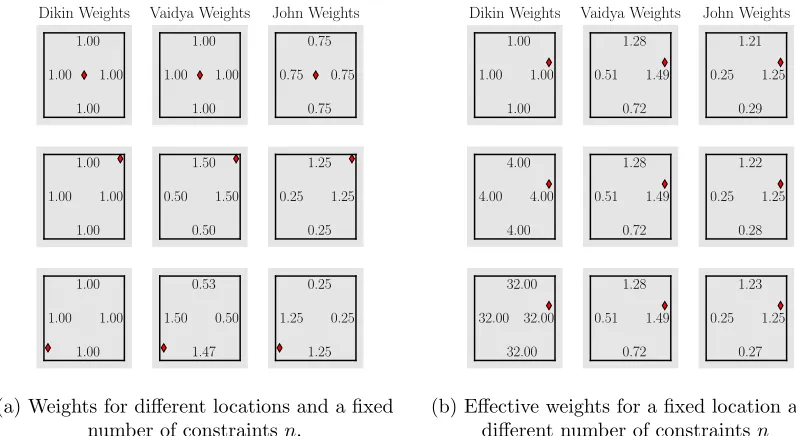
2.4 Visualization of three walks’ proposal distributions
In order to gain intuition about the three interior point based methods—namely, the Dikin, Vaidya and John walks—it is helpful to discuss how their underlying proposal distributions change as a function of the current pointx. All three walks are based on Gaussian proposal distributions with inverse covariance matrices of the general form
n X
i=1 wx,i
aia>i s2
x,i ,
wherewx,i >0 corresponds to a state-dependent weight associated with thei-th constraint. The Dikin walk uses the weightswx,i= 1; the Vaidya walk uses the weightswx,i=σx,i+βV;
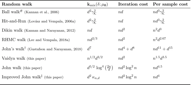
Random walk kmix(δ;µ0) Iteration cost Per sample cost
Ball walk#(Kannan et al., 2006) d2γ2
K nd nd3γK2
Hit-and-Run(Lov´asz and Vempala, 2006a) d2γ2
K nd nd3γK2
Dikin walk(Kannan and Narayanan, 2012) nd nd2 n2d3
RHMC walk(Lee and Vempala, 2018a) nd2/3 nd2 n2d2.67
John’s walk†(Gustafson and Narayanan, 2018) d7 nd4+d8 nd11+d15
Vaidya walk(this paper) n1/2d3/2 nd2 n1.5d3.5
John walk(this paper) d5/2 log4 2dn nd2log2n nd4.5
Improved John walk‡
(this paper) d2κn,d nd2log2n nd4
Table 1. Upper bounds on computational complexity of random walks on the polytope
K={x∈Rd|Ax≤b} defined by the matrix-vector pair (A, b)∈Rn×d×Rn with a
warm-start. For simplicity, here we ignore the logarithmic dependence on the warmness parameter and the toleranceδ. The iteration cost terms of ordernd2 arise from linear system solving,
using standard and numerically stable algorithms, fornequations inddimensions; algorithms with best possible theoretical complexityndωforω <1.373 are not numerically stable enough for practical use. #Mixing time of the Ball walk has been improved to
O d2γ
Kfor near isotropic convex bodies by Lee and Vempala (2018b) during the submission period of this paper. While ball walk, Hit-and-run are affected by the condition numberγKof the set, the Dikin and RHMC walks have quadratic dependence on the number of constraintsn. †John’s walk by Gustafson and Narayanan (2018) (based on the exact John ellipsoids) has linear dependence onnbut poor dependence ond. In contrast, the Vaidya walk has sub-quadratic dependence on n and significantly better dependence on d. Furthermore, the John walk (based on approximate John’s ellipsoids) analyzed in this paper has linear dependence with reasonable dependence on the dimensionsd. ‡The mixing time bound for the improved John walk with poly-logarithmic factorκn,d is conjectured.
the weightwx,i relative to the total weightPni=1wx,i signifies more importance for thei-th linear constraint for the pointx.
Figure 1a illustrates the difference in three weights as we move points inside the polytope [−1,1]2. When the pointxis in the middle of the unit square formed by the four constraints, all walks exhibit equal weight for every constraint. When the pointxis closer to the bottom-left boundary, the Vaidya and John weights assign larger weights to the bottom and the left constraints, while the weights for top and right constraints decrease. Note that the total sum of Vaidya weights and that of John weights remains constant independent of the position of the point x.
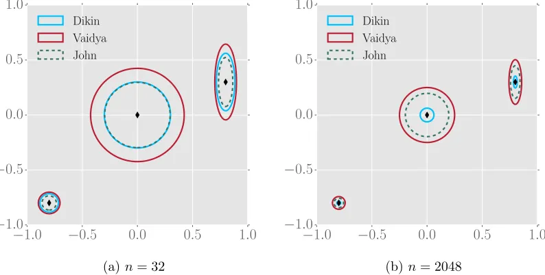
In Figure 1b-2b, we demonstrate that the Vaidya walk and the John walk are better at handling repeated constraints. Note that we can define the square [−1,1]2 as
[−1,1]2 =
x∈R2
Ax≤b, A=
1 0
0 1
−1 0
0 −1 , b=
1 1
1.00 1.00
1.00
1.00
Dikin Weights
1.00 1.00
1.00
1.00
Vaidya Weights
0.75 0.75
0.75
0.75
John Weights
1.00 1.00
1.00
1.00
0.50 1.50
1.50
0.50
0.25 1.25
1.25
0.25
1.00 1.00
1.00
1.00
1.50 0.53
0.50
1.47
1.25 0.25
0.25
1.25
(a) Weights for different locations and a fixed number of constraintsn.
1.00 1.00
1.00
1.00
Dikin Weights
0.51 1.28
1.49
0.72
Vaidya Weights
0.25 1.21
1.25
0.29
John Weights
4.00 4.00
4.00
4.00
0.51 1.28
1.49
0.72
0.25 1.22
1.25
0.28
32.00 32.00
32.00
32.00
0.51 1.28
1.49
0.72
0.25 1.23
1.25
0.27
(b) Effective weights for a fixed location and different number of constraintsn
Figure 1. Visualization of the weights on the square with repeated constraints Sn/4 for
the different random walks. The number mentioned next to the boundary lines denotes the effective weight for the locationx (denoted by diamond) for the corresponding constraint.
(a)n= 4 is common across rows andx= (0,0) for the top row, (0.9,0.9) for the middle and (−0.9,−0.7) for the bottom row. The Dikin weights are independent ofx, the Vaidya and the John weights for a constraint increase if the locationxis closer to it. (b)x= (0.85,0.30) is common across rows, andn= 4 for the top row,n= 16 for the middle andn= 128 for the bottom row. The effective Dikin weight for each constraint increases linearly withnbut for the Vaidya and John walk adaptively, the weights get adjusted such that the sum of their weights is always of the order of the dimensiond.
Simply repeating the rows of the matrix A several times changes the mathematical for-mulatiton of the polytope, but does not change the shape of the polytope. We define the square with constraints repeatedn/4 timesSn/4 as
Sn/4 = x∈R
2
An/4x≤bn/4, An/4 =
A .. . ×(n/4)
, bn/4 =
b .. . ×(n/4)
,
(14)
number of constraints is large. Nonetheless, such a claim is only based on heuristics and is presented simply to provide an intuition that the new ellipsoids are better behaved than Dikin ellipsoids and thereby motivated the design of the new random walks.
−1.0 −0.5 0.0 0.5 1.0
−1.0
−0.5 0.0 0.5 1.0
Dikin Vaidya John
(a)n= 32
−1.0 −0.5 0.0 0.5 1.0
−1.0
−0.5 0.0 0.5 1.0
Dikin Vaidya John
(b)n= 2048
Figure 2. Visualization of the proposal distribution on the square with repeated constraints
Sn/4 for the different random walks. (a, b) Unit ellipsoids associated with the covariances
of the random walks at different states x on the square with repeated constraints Sn/4.
Clearly, all these ellipsoids adapt to the boundary but increasing nhas a profound impact on the volume of the Dikin ellipsoids and comparatively less impact on the Vaidya and John ellipsoids.
3. Main results
With the basic background in place, we now describe the algorithms more precisely and state upper bounds on the mixing time of the Vaidya and John walks. In Section 3.4, we propose a variant of the John walk, known as the improved John walk, and conjecture that it has a better mixing time bound than that of the John walk.
3.1 Vaidya and John walks
In this subsection, we formally define the Vaidya and John walks. In Algorithm 1 and Algorithm 2, we summarize the steps of the Vaidya walk and the John walk.
Vaidya walk: The Vaidya walk with radius parameter r > 0, denoted by VW(r) for short, is defined by a Gaussian proposal distribution denoted as PV
N x,√r2 ndVx
−1. In analytic terms, the proposal density atx is given by
pV
x(z) :=pVaidya(r)(x, z) = p
detVx
nd 2πr2
d/2
exp −
√
nd
2r2 (z−x) >V
x(z−x) !
. (15)
As the target distribution for our walk is the uniform distribution onK, the proposal step is followed by an accept-reject step as described in Section 2.1 (equation 1). Thus the overall transition distribution for the walk at statex is defined by a density given by
qVaidya(r)(x, z) =
(
min{pV
x(z), pVz(x)}, z∈ Kand z6=x,
0, z /∈ K,
and a probability mass at x, given by 1−Rz∈Kmin{px(z), pz(x)}dz. We use TVaidya(r) to denote the resulting transition operator for the Vaidya walk with parameter r.
Algorithm 1:Vaidya Walk with parameterr (VW(r))
Input: Parameterr andx0∈int (K)
Output: Sequencex1, x2, . . .
1 fori= 0,1, . . .do
2 With probability 12 stay at the current state: xi+1←xi %lazy step
3 With probability 12 perform the following update:
4 Proposal step: Drawzi+1 ∼ N
xi, r 2
(nd)1/2V−
1
xi
5 Accept-reject step:
6 if zi+1∈ K/ thenxi+1←xi %reject an infeasible proposal
7 else
8 compute αi+1= min1, pzi+1(xi+1)/pxi+1(zi+1)
9 With probabilityαi+1 accept the proposal: xi+1←zi+1
10 With probability1−αi+1 reject the proposal: xi+1←xi
11 end
John walk: The John walk is similar to the Vaidya walk except that the proposals at state x∈int (K) are generated from the multivariate Gaussian distributionN x, r2
d3/2·log4 2(2n/d)
Jx−1
, where the matrix Jx is defined by equation (11), and r > 0 is a constant. The proposal distribution at x ∈ int (K) is denoted as PJ
x. The proposal step is then followed by an accept-reject step similarly defined as in the Vaidya walk. We use TJohn(r) to denote the resulting transition operator for the John walk with parameterr.
3.2 Mixing time bounds for warm start
We are now ready to state an upper bound on the mixing time of the Vaidya walk. In this and other theorem statements, we usecto denote a universal positive constant. Recall thatπ∗ denotes the uniform distribution on the polytopeK, and, thatT
Vaidya(r) denotes the
Algorithm 2:John Walk with parameterr (JW(r))
Input: Parameterr andx0∈int (K)
Output: Sequencex1, x2, . . .
1 fori= 0,1, . . .do
2 With probability 12 stay at the current state: xi+1←xi %lazy step
3 With probability 12 perform the following update:
4 Proposal step: Drawzi+1∼ N
xi, r 2 d3/2J−
1
xi
%this step is different than the Vaidya walk
5 Accept-reject step:
6 if zi+1∈ K/ thenxi+1←xi %reject an infeasible proposal
7 else
8 compute αi+1= min1, pzi+1(xi+1)/pxi+1(zi+1)
9 With probabilityαi+1 accept the proposal: xi+1←zi+1
10 With probability1−αi+1 reject the proposal: xi+1←xi
11 end
Theorem 1 Let µ0 be any distribution that is M-warm with respect to π∗ as defined in
equation (Warm-Start). For any δ ∈ (0,1], the Vaidya walk with parameter rV = 10−4
satisfies
kTk
Vaidya(rV)(µ0)−π
∗
kTV ≤δ for all k≥cn1/2d3/2 log
√
M δ
!
. (16)
The proof of Theorem 1 is provided in Section 5. Theorem 1 precisely quantifies the depen-dence of mixing time of the Vaidya walk on many parameters of interest such as dimension d, number of constraintsn, the error toleranceδ and the warmnessM. The specific choice rV = 10−4 is for theoretical purposes; in practice, we find that substantially larger values
can be used.2 Our upper bound for the mixing time of the Vaidya walk has O(pn/d) improvement over the current best upper bound for the mixing time of the Dikin walk. In Section 4.1, we show that the per iteration cost for the two walks is of the same order. Since n≥dfor closed polytopes inRd, the effective cost until convergence (iteration com-plexity multiplied by number of iterations required) for the Vaidya walk is at least of the same order as of the Dikin walk, and significantly smaller when n d. Comparing the provable mixing time upper bounds, the Vaidya walk has an advantage over the Dikin walk for the problems where the number of constraints is significantly larger than the number of variables involved. Our simulations also confirm this theoretical finding.
Let us now state our result for the mixing time of the John walk:
2. A larger than optimalr leads to an undesirable high rejection rate. In practice, we can fine tune r
by performing a binary search over the interval [10−4,1] and keeping track of the rejection rate of the
Theorem 2 Suppose that n ≤ exp(√d), and let µ0 be any distribution that is M-warm
with respect toπ∗. Then for anyδ ∈(0,1], the John walk with parameterr
J= 10−5 satisfies
kTJohnk (rJ)(µ0)−π
∗
kTV≤δ for allk≥c d
2.5 log4n d
log
√
M δ
! .
The proof of Theorem 2 is provided in Appendix D. Again the specific choice of rJ= 10−5
is for theoretical purpose; in practice larger choices are possible. Note that the mixing time bound for the John walk depends only on the number of constraints n via a logarithmic factor, and so is almost independent of n. Consequently, it has a mixing time that is polynomial in deven if the number of constraints n scales exponentially in √d. Further, we show in Section 4.1 that the cost to execute one step of the John walk is of the same order as of the Dikin walk up to a poly-logarithmic factor in n. Thus, using John walk, we obtain improved mixing time bounds for the case whennd2.
3.3 Mixing time bounds from deterministic start
The mixing time bounds in Theorem 1 and 2 depend on the warmness M of the initial distribution. In some applications, it may not be easy to find an M-warm initial distribu-tion. In such cases, we can consider starting the random walk from a deterministic point x0 ∈int (K) that is not too close to the boundary ∂K. Indeed, such a point can be found using standard optimization methods—e.g., using a Phase-I method for Newton’s algorithm (see Boyd and Vandenberghe, 2004, Section 11.5.4).
Given such a deterministic initialization, our mixing time guarantees depend on the distance of the starting point from the boundary. This dependence involves the following notion of s-centrality:
Definition 3 A point x ∈ int (K) is called s-central if for any chord ef with end points
e, f ∈∂K passing throughx, we have ke−xk2/kf−xk2 ≤s.
Assuming that it is started at ans-central pointx0, the Dikin walk (Kannan and Narayanan, 2012, algorithm in section 2.1) has a polynomial mixing time. The authors showed that when the walk moves to a new state for the first time, the distribution of the iterate is
O (√ns)d-warm with respect to the distribution3π∗. Since only constant number of steps is required to get a warm start, for a deterministic start, we can just use the Dikin walk in the beginning to provide a warm start to the Vaidya (or John) walk. This motivates us to define the following hybrid walk.
Given ans-central pointx0, simulate the Dikin walk until we observe a new state. Note that due tolaziness and the accept-reject step, the chain can stay at the starting point for several steps before making the first move a new state. Letk1 denote the (random) number of steps taken to make the first move to a new state. Afterk1 steps, we run the walk VW(r) withxk1 as the initial point. We call such a walk ass-central Dikin-start-Vaidya-walk with
parameterr. LetTDikindenote the transition kernel of the Dikin walk stated above. Then, we have the following mixing time bound for this hybrid walk.
Corollary 4 Any s-central Dikin-start-Vaidya-walk with parameter r= 10−4 satisfies
kTk
Vaidya(r) TDikink1 (δx0)
−π∗kTV≤δ for allk≥cn1/2d5/2 log
ns δ
,
where k1 is a geometric random variable with E[k1] ≤c0, and c, c0 > 0 are universal
con-stants.
The mixing rate is logarithmic innsand has an extra factor ofdcompared to the bounds in Theorem 1. However, guaranteeing a warm start for a general polytope is hard but obtaining a central point involves only a few steps of optimization. Consequently, the hybrid walk and the guarantees from Corollary 4 come in handy for all such cases. Once again we observe that the upper bounds for mixing time are improved by a factor ofO(pn/d) when compared to the Dikin walk from ans-central start (Kannan and Narayanan, 2012; Narayanan, 2016) which had a mixing time of O nd2. The proof follows immediately from Theorem 1 by Kannan and Narayanan (2012) and Theorem 1 of this paper and is thereby omitted.
In a similar fashion, we can provide a polynomial time guarantee for a modified John walk from a deterministic start. We can consider a hybrid random walk that starts at an s-central point, simulates the Dikin walk until it makes the first move to a new state, and from there onwards simulates the John walk. Such a chain would have a mixing time of
O d3.5poly-log(n, d, s). For brevity, we omit a formal statement of this result. 3.4 Conjecture on improved John walk
From our analysis, we suspect that it is possible to improve the mixing time bound of
O d2.5poly-log(n/d)in Theorem 2 by considering a variant of the John walk. In particular, we conjecture that a random walk with proposal distribution given byN x, r2
d·poly-log(n/d)Jx −1 for a suitable choice of r has an O d2poly-log(n/d) mixing time from a warm start. We refer to this random walk as theimproved John walk, and denote its transition operator by
TJohn+. Let us now give a formal statement of our conjecture on its mixing rate.
Conjecture 5 Let µ0 be any M-warm distribution. Then for any δ ∈(0,1], the improved
John walk with parameter r=r0, satisfies the bound
kTJohnk +(µ0)−π
∗
kTV ≤δ for allk≥c d
2 logc0
2
2n d
log
√
M δ
! ,
where r0, c, c0 are universal constants.
Note that this conjecture involves quadratic (degree two) scaling in d; this exponent of two matches the sum of exponents fordandnin the mixing time bounds for both the Dikin and Vaidya walks from a warm-start. Consquently, the improved John walk would have better performance than the Dikin, Vaidya and John walks for almost all ranges of (n, d), apart from possible poly-logarithmic factors in the ration/d.
3.5 Proof sketch
main proof relies on the work by Lov´asz (1999) that characterizes the conductance of Markov chains on a convex set using Hilbert metric. Precisely, Lov´asz (1999) showed that a Markov chain has good conductance if it makes jumps to regions with large overlaps from two nearby points and the mixing time depends inversely on the maximum Hilbert metric between such nearby points. Using this argument, it remains to make sure that the ellipsoid radius is chosen properly such that the ellipsoids remain inside the polytope and the ellipsoids corresponding to two different points x and y overlap a lot even if the points x and y are relatively far apart.
The conductance-based argument has been used for analyzing the ball walk (Lov´asz and Simonovits, 1990, 1993), Hit-and-run (Lov´asz, 1999; Lov´asz and Vempala, 2006a) and the Dikin walk (Kannan and Narayanan, 2012; Narayanan, 2016; Sachdeva and Vishnoi, 2016). We refer the reader to the survey by Vempala (2005) for a thorough discussion about the relation between the conductance and mixing time for Markov chains. Our proof techniques share a few features with the recent analyses of the Dikin walk by Kannan and Narayanan (2012) and Sachdeva and Vishnoi (2016). However, new technical ideas are needed in order to handle the state-dependent weights σx and ζx, as defined in equations (9b) and (12) respectively, that underlie the proposal distributions for the Vaidya and John walks. Note that these techniques are not present in the analysis of the Dikin walk, which is based on constant weights.
Specifically, we present the proof of Theorem 1 on the mixing time of the Vaidya walk in Section 5 and defer the intermediate technical results to Appendix A, B and C. We present the proof of Theorem 2 (mixing time bound for the John walk) in Appendix D and provide related auxiliary results and their proofs in Appendices E, F, G, H and I. As alluded to earlier, to keep the paper self-contained, we provide the proof of Lov´asz’s Lemma in Appendix J.
4. Numerical experiments
In this section, we first analyze the per-iteration cost to implement of three walks. We show that while the Dikin walk has the best per-iteration cost, the per-iteration cost of the Vaidya walk is only twice of that of Dikin walk and the per-iteration cost of the John walk is only of order log2(2n/d) larger. Second, we demonstrate the speed-up gained by the Vaidya walk over the Dikin walk for a warm start on different polytopes.
4.1 Per iteration cost
We now show that the per iteration cost of the Dikin, Vaidya and John walks is of the same order. The proposal step of Vaidya walk requires matrix operations like matrix inversion, matrix multiplication and singular value decomposition (SVD). The accept-reject step re-quires computation of matrix determinants, besides a few matrix inverses and matrix-vector products. The complexity of all aforementioned operations is O nd2. Thus, per iteration computational complexity for the Vaidya walk is O nd2.4
4. In theory, the matrix computations for the Dikin walk can be carried out in timendν for an exponent
Both the Dikin and Vaidya walks requires an SVD computation for inverting the Hessian of Dikin barrier ∇2F
x. In addition for the Vaidya walk, we have to invert the matrix Vx, which leads to almost twice the computation time of the Dikin walk per step. This difference can be observed in practice.
For the John walk, we need to compute the weights ζx at each point which involves solving the program (12). Lee and Sidford (2014) argued that the convex program (12) for obtaining John walk’s weights is strongly convex with a suitably chosen norm. They proved that solving this program requires log2nnumber of gradient steps, where the computational complexity of each gradient step is equivalent to that of solving an n×d linear system (O nd2using a numerically stable routine). Thus, the overall cost for the John walk is of the same order as of the Dikin walk up to a poly-logarithmic factor in the pair (n, d).
In practice, for the John walk, the combined effect of logarithmic factors in the number of steps and the cost to implement each step cannot be ignored. This extra factor becomes a bottleneck for the overall run time for the convergence of the Markov chain. Consequently, the John walk is not suitable for polytopes with moderate values ofnandd, and its mixing time bounds are computationally superior to the Dikin and Vaidya walks only for the polytopes withnd1.
4.2 Simulations
We now present simulation results for the random walks in Rd for d = 2,10 and 50 with initial distributionµ0=N(0, σd2Id) and target distribution being uniform, on the following polytopes:
Set-up 1 : The set [−1,1]2 defined by different number of constraints.
Set-up 2 : The set [−1,1]dford∈ {2,3,4,5,6,7} forn={2d,2d2,2d3} constraints. Set-up 3 : Symmetric polytopes inR2 with n-randomly-generated-constraints.
Set-up 4 : The interior of regularn-polygons on the unit circle.
Set-up 5 : Hyper cube [−1,1]d ford= 10 and 50.
We choose σdsuch that the warmness parameterM is bounded by 100. We provide imple-mentations of the Dikin, Vaidya and John walks in python and a jupyter notebook at the github repository https://github.com/rzrsk/vaidya-walk.
We use the following three ways to compare the convergence rate of the Dikin and the Vaidya walks: (1) comparing the approximate mixing time of a particular subset of the polytope—smaller value is associated with a faster mixing chain; (2) comparing the plot of the empirical distribution of samples from multiple runs of the Markov chain after k steps—if it appears more uniform for smallerk, the chain is deemed to be faster; and (3) contrasting the sequential plots of one dimensional projection of samples for a single long run of the chain—less smooth plot is associated with effective and fast exploration leading to a faster mixing (Yu and Mykland, 1998). Note that MCMC convergence diagnostics is a hard problem, especially in high dimensions, and since the methods outlined above are heuristic in nature we expect our experiments to not fully match our theoretical results.
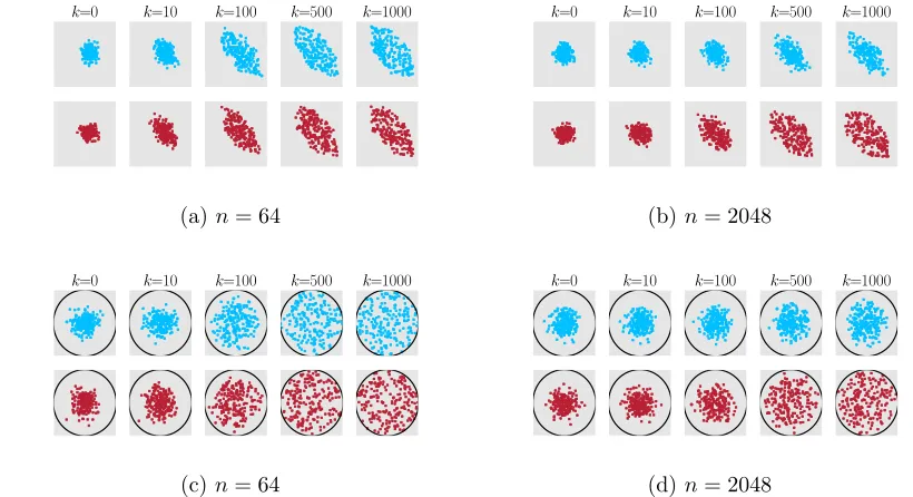
then run the Dikin and Vaidya walks with the new A. Given the larger number of con-straints, our theory predicts that the random walks should mix more slowly. In Figure 3c and 3d, we plot the empirical distribution obtained by the Dikin walk and Vaidya walk, starting from 200 i.i.d initial samples, forn= 64 and 2048. The empirical distribution plot shows that having large n significantly slows the mixing rate of the Dikin walk, while the effect on the Vaidya walk is much less. Further, we also plot the scaling of the approxi-mate mixing time ˆkmix (defined below) for this simulation as a function of the number of constraints n in Figure 3b. For Set-up 2, we plot ˆkmix as a function of the dimensionsd in Figures 3e-3g, for the random walks on [−1,1]dwhere the hypercube is parametrized by different number of constraintsn∈ {2d,2d2,2d3}. The approximate mixing time is defined with respect to the set Sd = {x ∈ Rd| |xi| ≥ cd ∀i ∈ [d]} where cd is chosen such that π∗(Sd) = 1/2. In particular, for a fixed value of n, let ˆTk denote the empirical measure afterk-iterations across 2000 experiments. The approximate mixing time ˆkmixis defined as
ˆ
kmix:= min
k
π∗(Sd)−Tˆk(Sd)≤ 1 20
, (17)
We choose such a set since the set covers the regions near to the boundary of the poly-tope which are not covered well by the chosen initial distribution. We make the following observations:
1. The slopes of the best-fit lines, for ˆkmix versusn in the log-log plot in Figure 3b, are 0.88 and 0.45 for Dikin and Vaidya walks respectively. This observation reflects a near-linear and sub-linear dependence on n for a fixed dfor the mixing time of the Dikin walk and the Vaidya walk respectively.
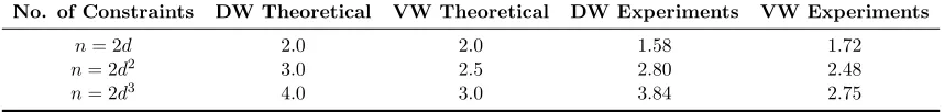
2. In Figures 3e-3g, once again we observe a more significant effect of increasing the number of constraints on the approximate mixing time ˆkmix. We list the slopes of the best fit lines on these log-log plots in Table 2. These slopes correspond to the exponents fordfor the approximate mixing time. From the table, we can observe that these experiments agree with the mixing time bounds of O(nd) for the Dikin walk and O n0.5d1.5 for the Vaidya walk.
No. of Constraints DW Theoretical VW Theoretical DW Experiments VW Experiments
n= 2d 2.0 2.0 1.58 1.72
n= 2d2 3.0 2.5 2.80 2.48
n= 2d3 4.0 3.0 3.84 2.75
Table 2. Value of the exponent of dimensions dfor the theoretical bounds on mixing time
and the observed approximate mixing time of the Dikin walk (DW) and the Vaidya walk (VW) for [−1,1]d described byn= 2d,2d2,2d3 constraints. The theoretical exponents are
based on the mixing time bounds ofO(nd) for the Dikin walk andO n0.5d1.5for the Vaidya
walk. The experimental exponents are based on the results from the simulations described
in Set-up 2 in Section 4.2. Clearly, the exponents observed in practice are in agreement
with the theoretical rates and imply the faster convergence of the Vaidya walk compared to the Dikin walk for large number of constraints.
random variables from [0,1] and then flip the sign of both of them with probability 1/2 and assign these values to the vectorai. The resulting polytope is always a subset of the square
K= [−1,1]2 and contains the diagonal line connecting the points (−1,1) and (1,−1). From Figure 4a-4b, we observe that while there is no clear winner for the casen= 64, the Vaidya walk mixes mixes significantly faster than the Dikin walk for the polytope defined by 2048 constraints.
In Set-up 4, the constraint set is the regularn-polygons inscribed in the unit circle. A similar observation as inSet-up 3can be made from Figure 4c-4d: the Vaidya walk mixes at least as fast as the Dikin walk and mixes significantly faster for largen.
In Set-up 5, we examine the performance of the Dikin walk and the Vaidya walk on hyper-cube [−1,1]d ford= 10,50. We plot the one dimensional projections onto a random normal direction of all the samples from a single run up to 10,000 steps. The Vaidya sequential plot looks more jagged than that of the Dikin walk for d = 10, n = 5120. For other cases, we do not have a clear winner. Such an observation is consistent with the
O(pn/d) speed up of the Vaidya walk which is apparent when the ration/dis large.
5. Proofs
We begin with auxiliary results in Section 5.1 which we use then to prove Theorem 1 in Section 5.2. Proofs of the auxiliary results are in Sections 5.3 and 5.4, and we defer other technical results to appendices.
5.1 Auxiliary results
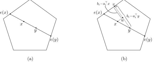
Our proof proceeds by formally establishing the following property for the Vaidya walk: if two points are close, then their one-step transition distribution are also close. Consequently, we need to quantify the closeness between two points and the associated transition distri-butions. We measure the distance between two points in terms of the cross ratio that we define next. For a given pair of pointsx, y∈ K, lete(x), e(y)∈∂K denote the intersection of the chord joining x and y with K such that e(x), x, y, e(y) are in order (see Figure 6a). The cross-ratiodK(x, y) is given by
dK(x, y) := ke(x)−e(y)k2kx−yk2
ke(x)−xk2ke(y)−yk2. (18)
The ratiodK(x, y) is related to the Hilbert metric onK, which is given by log (1 +dK(x, y)); see the paper by Bushell (1973) for more details.
Consider a lazy reversible random walk on a bounded convex set K with transition operator T defined via the mapping µ0 7→ µ0/2 + ˜T(µ0)/2 and stationary with respect to the uniform distribution on K (denoted by π∗). (Recall that δx denote the dirac-delta distribution with unit mass at x.) The following lemma gives a bound on the mixing-time of the Markov chain.
Lemma 6 (Lov´asz’s Lemma) Suppose that there exist scalarsρ,∆∈(0,1) such that
−1.0 −0.5 0.0 0.5 1.0
−1.0
−0.5 0.0 0.5 1.0
initial
−1.0 −0.5 0.0 0.5 1.0
−1.0
−0.5 0.0 0.5 1.0
target
(a)
101 102 103
n
101
102
103
ˆkmix
Dikin Vaidya
(b)
k=10 k=100 k=500 k=1000
(c)n= 64
k=10 k=100 k=500 k=1000
(d)n= 2048
100 101
d
102
103
104
ˆkmix
Dikin Vaidya
(e)n= 2d
100 101
d
102
103
104
105
ˆkmix
Dikin Vaidya
(f) n= 2d2
100 101
d
102
103
104
105
ˆkmix
Dikin Vaidya
(g)n= 2d3
Figure 3. Comparison of the Dikin and Vaidya walks on the polytope K = [−1,1]2. (a)
Samples from the initial distribution µ0 = N(0,0.04I2) and the uniform distribution on
[−1,1]2. (b) Log-log plot of ˆk
mix (17) versus the number of constraints (n) for a fixed
dimensiond= 2. (c, d)Empirical distribution of the samples for the Dikin walk (blue/top rows) and the Vaidya walk (red/bottom rows) for different values of n at iteration k = 10,100,500 and 1000. (e, f, g) Log-log plot of ˆkmixvs the dimensiond, forn∈ {2d,2d2,2d3}
for d∈ {2,3,4,5,6,7}. The exponents from these plots are summarized in Table 2. Note that increasing the number of constraintsn has more profound effect on the Dikin walk in almost all the cases.
Then for every distributionµ0that isM-warm with respect toπ∗, the lazy transition operator
T satisfies
kTk(µ0)−π∗kTV≤
√
Mexp
−k∆ 2ρ2 4096
k=0 k=10 k=100 k=500 k=1000
(a)n= 64
k=0 k=10 k=100 k=500 k=1000
(b)n= 2048
k=0 k=10 k=100 k=500 k=1000
(c)n= 64
k=0 k=10 k=100 k=500 k=1000
(d)n= 2048
Figure 4. Empirical distribution of the samples from 200 runs for the Dikin walk (blue/top
rows) and the Vaidya walk (red/bottom rows) at different iterations k. The 2-dimensional polytopes considered are: (a, b)random polytopes with n-constraints, and (c, d) regular n-polygons inscribed in the unit circle. For both sets of cases, we observe that highernslows down the walks, with visibly more effect on the Dikin walk compared to the Vaidya walk.
0 2000 4000 k→ 6000 8000 10000
−6 −3 0 3 6
Vaidya Dikin
0 2000 4000 k→ 6000 8000 10000
−4.00 −2.25 −0.50 1.25 3.00
Vaidya Dikin
0 2000 4000 k→ 6000 8000 10000
−3.00 −1.25 0.50 2.25 4.00
Vaidya Dikin
(a)d= 10
0 2000 4000 k→ 6000 8000 10000
−8.0 −3.5 1.0 5.5 10.0
Vaidya Dikin
0 2000 4000 k→ 6000 8000 10000
−6 −3 0 3 6
Vaidya Dikin
0 2000 4000 k→ 6000 8000 10000
−8.0 −4.5 −1.0 2.5 6.0
Vaidya Dikin
(b)d= 50
Figure 5. Sequential plots of a one-dimensional random projection of the samples on the
hyperboxK= [−1,1]d, defined bynconstraints. Each plot corresponds to one long run of the Dikin and Vaidya walks, and the projection is taken in a direction chosen randomly from the sphere. (a) Plots for d= 10 and n∈ {20,640,5120}. (b) Plots for d= 50 and n∈ {100,400,1600}. Relative to the Dikin walk, the Vaidya walk has a more jagged plot for pairs (n, d) in which the ration/dis relatively large: for instance, see the plots corresponding to (n, d) = (640,10) and (5120,10). The same claim cannot be made for pairs (n, d) for which the ration/dis relatively small; e.g., the plot with (n, d) = (20,10). These observations are consistent with our results that the Vaidya walk mixes more quickly by a factor of order
x
y
e(x)
e(y)
(a)
x
y
e(x)
e(y)
)
{
bi a>iy
bi a>ix
u v
(b)
Figure 6. Polytope K = {x ∈ Rd|Ax ≤ b}. (a) The points e(x) and e(y) denote the
intersection points of the chord joiningxandywithKsuch thate(x), x, y, e(y) are in order. (b) A geometric illustration of the argument (23). It is straightforward to observe that
kx−yk2/ke(x)−xk2=ku−yk2/ku−vk2=a> i (y−x)
/ bi−a>i x
.
This result is implicit in the paper by Lov´asz (1999), though not explicitly stated. In order to keep the paper self-contained, we provide a proof of this result in Appendix J.
Our proof of Theorem 1 is based on applying Lov´asz’s Lemma; the main challenge in our work is to establish that our random walks satisfy the condition (19a) with suitable choices of ∆ andρ. In order to proceed with the proof, we require a few additional notations. Recall that the slackness at xwas defined as sx:= (b1−a>1x, . . . , bn−a>nx)>. For allx∈int (K), define theVaidya local norm of v at x as
kvkV x :=
V1/2
x v
2 = v u u t
n X
i=1
(σx,i+βV)
(a> i v)2 s2
x,i
, (20a)
and theVaidya slack sensitivity at x as
θVx :=
a1 sx,1
2 Vx
, . . . ,
an sx,n
2 Vx
!>
= a
> 1Vx−1a1
s2 x,1
, . . . ,a > nVx−1an
s2 x,n
!>
. (20b)
Similarly, we define theJohn local norm of v atx and theJohn slack sensitivity at x as
kvkJ x :=
J1/2
x v
2 and θJx :=
a1 sx,1
2 Jx
, . . . ,
an sx,n
2 Jx
!>
. (20c)
The following lemma provides useful properties of the leverage scoresσxfrom equation (9b), the weights ζx obtained from solving the program (12), and the slack sensitivities θVx and θJx.
Lemma 7 For any x∈int (K), the following properties hold:
(a) σx,i ∈[0,1] for alli∈[n],
(c) θVx,i∈ h
0,pn/difor all i∈[n],
(d) ζx,i∈[βJ,1 +βJ]for all i∈[n],
(e) Pni=1ζx,i = 3d/2, and
(f ) θJx,i∈[0,4] for alli∈[n].
We prove this lemma in Section 5.3.
LetPV
x to denote the proposal distribution of the random walk VW(r) at statex. Next, we state a lemma that shows that if two pointsx, y∈int (K) are close in Vaidya local norm at x, then for a suitable choice of the parameter r, the proposal distributions PV
x and PyV are close. In addition, we show that the proposals are accepted with high probability at any point x∈int (K). To establish the latter result, we now define the non-lazy transition operator of the Vaidya walk. Since the Vaidya walk is lazy with probability 1/2, there exists a valid (non-lazy) transition operator ˜TVaidya(r) such that for any distribution µ0, we have
TVaidya(r)(µ0) =µ0/2 + ˜TVaidya(r)(µ0)/2.
We call ˜TVaidyathe non-lazy transition operator for the Vaidya walk. Note that the one-step
non-lazy transition distribution ˜TVaidya(r)(δx) denotes the distribution of proposals after the accept-reject step if the chain was not lazy. Thus to establish that proposals are accepted with high probability, it suffices to establish that the transition distribution ˜TVaidya(r)(δx) at any point x ∈ K is close to the proposal distribution PV
x. We now state these two results formally:
Lemma 8 There exists a continuous non-decreasing function f : [0,1/4] → R+ with f(1/15)≥10−4 such that for any ∈(0,1/15], the random walk VW(r) with r ∈[0, f()]
satisfies
kPV
x − P
V
ykTV≤ ∀ x, y∈int (K) s.t. kx−ykVx ≤
r
2(nd)1/4 , and (21a)
kT˜Vaidya(r)(δx)− P V
xkTV≤5 ∀ x∈int (K). (21b)
See Section 5.4 for the proof of this lemma.
With these lemmas in hand, we are now equipped to prove Theorem 1. To simplify notation, for the rest of this section, we adopt the shorthands Tx = ˜TVaidya(r)(δx), Px = PxV and
k·kVx =k·kx.
5.2 Proof of Theorem 1
In order to invoke Lov´asz’s Lemma for the random walk VW(10−4), we need to verify the condition (19a) for suitable choices ofρ and ∆. Doing so involves two main steps:
(A): First, we relate the cross-ratio dK(x, y) to the local norm (20a) at x.
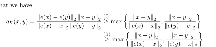
Step (A): We claim that for allx, y∈int (K), the cross-ratio can be lower bounded as
dK(x, y)≥ √1
2dkx−ykx. (22)
Note that we have
dK(x, y) = ke(x)−e(y)k2kx−yk2
ke(x)−xk2ke(y)−yk2 (i)
≥max
kx−yk2
ke(x)−xk2
, kx−yk2
ke(y)−yk2
(ii)
≥ max
kx−yk2
ke(x)−xk2,
kx−yk2
ke(y)−xk2
,
where step (i) follows from the inequalityke(x)−e(y)k2 ≥max{ke(y)−yk2,ke(x)−xk2}; and step (ii) follows from the inequality ke(x)−xk2 ≤ ke(y)−xk2. Furthermore, from Figure 6b, we observe that
max
kx−yk2
ke(x)−xk2
, kx−yk2
ke(y)−xk2
= max i∈[n] a
>
i (x−y) sx,i
. (23)
This argument of equation (14) has also been used (Sachdeva and Vishnoi, 2016, lemma 9). Note that maximum of a set of non-negative numbers is greater than the mean of the numbers. Combining this fact with properties (a) and (b) from Lemma 7, we find that
dK(x, y)≥
v u u
tPn 1
i=1(σx,i+βV)
n X
i=1
(σx,i+βV)
(a>
i (x−y))2 s2
x,i
= kx√−ykx
2d ,
thereby proving the claim (22).
Step (B): By the triangle inequality, we have
kTx−TykTV≤ kTx− PxkTV+kPx− PykTV+kPy−TykTV.
Thus, for any (r, ) such that∈[0,1/15] and r≤f(), Lemma 8 implies that
kTx−TykTV≤11, ∀x, y∈int (K) such that kx−ykx≤
r 2(nd)1/4.
Consequently, the walk VW(r) satisfies the assumptions of Lov´asz’s Lemma with
∆ := √1
2d· r
2(nd)1/4 and ρ:= 1−11. Since f(1/15)≥10−4, we can set = 1/15 andr = 10−4, whence
∆2ρ2= (1−11) 22r2 8d√nd =
42 152
1 152
1 10−8 ·
1
d√nd ≥10
−12 1 d√nd.
5.3 Proof of Lemma 7
In order to prove part (a), observe that for anyx∈int (K), the Hessian∇2F x :=
Pn
i=1aia>i /s2x,i is a sum of rank one positive semidefinite (PSD) matrices. Also, we can write∇2F
x =A>xAx where
Ax :=
a>1/sx,1 .. . a>n/sx,n
.
Since rank(Ax) = d, we conclude that the matrix ∇2Fx is invertible and thus, both the matrices∇2F
x and ∇2Fx −1
are PSD. Sinceσx,i =a>i ∇2Fx −1
ai/s2x,i, we haveσx,i≥0. Further, the fact that aia>i /s2x,i ∇2Fx implies thatσx,i ≤1.
Turning to the proof of part (b), from the equality trace(AB) = trace(BA), we obtain
n X
i=1
σx,i = trace n X
i=1 a>
i ∇2Fx −1
ai s2
x,i
!
= trace ∇2F x
−1Xn i=1
aia>i s2
x,i !
= trace(Id) =d.
Now we prove part (c). Using the fact thatσx,i≥0, and an argument similar to part (a) we find that that the matrices Vx and Vx−1 are PSD. Since θVx,i = a
>
i Vx−1ai/s2x,i, we have θVx,i≥0. It is straightforward to see thatβV∇2FxVx which implies thatθVx,i ≤σx,i/β. Further, we also have (σx,i+βV)
aia>i
s2
x,i Vx and whence θVx,i ≤1/(σx,i+βV). Combining the two inequalities yields the claim.
The other parts of the Lemma follow from Lemma 13, 14 and 15 by Lee and Sidford (2014) and are thereby omitted here.
5.4 Proof of Lemma 8
We prove the lemma for the following function
f() := min
1
201 +√2 log12 4
,p18 log(2/) ,
r
86√3χ2
,
22p5/3χ3 ,
r
50√105χ4 ,
(24)
where χk = (2e/k·log (4/))k/2 for k= 2,3 and 4. A numerical calculation shows that f(1/15)≥10−4.
5.4.1 Proof of claim (21a)
In order to bound the total variation distancekPx− PykTV, we apply Pinsker’s inequality,
which provides an upper bound on the TV-distance in terms of the KL divergence:
kPx− PykTV≤
q
2 KL(PxkPy).
![Figure 3. Comparison of the Dikin and Vaidya walks on the polytopethat increasing the number of constraints[dimension10forrows) and the Vaidya walk (red/bottom rows) for different values of K = [−1, 1]2](https://thumb-us.123doks.com/thumbv2/123dok_us/9781279.1963456/21.612.102.514.55.471/comparison-polytopethat-increasing-constraints-dimension-forrows-vaidya-dierent.webp)