Identifying a Minimal Class of Models for High–dimensional
Data
Daniel Nevo [email protected]
Department of Statistics
The Hebrew University of Jerusalem Mt. Scopus, Jerusalem, Israel and
Current address: Departments of Biostatistics and Epidemiology Harvard T.H. Chan School of Public Health
Boston, MA 02115, USA
Ya’acov Ritov [email protected]
Department of Statistics
The Hebrew University of Jerusalem Mt. Scopus, Jerusalem, Israel and
Department of Statistics University of Michigan
Ann Arbor, MI 48109–1107, USA
Editor:Nicolai Meinshausen
Abstract
Model selection consistency in the high–dimensional regression setting can be achieved only if strong assumptions are fulfilled. We therefore suggest to pursue a different goal, which we call a minimal class of models. The minimal class of models includes models that are similar in their prediction accuracy but not necessarily in their elements. We suggest a random search algorithm to reveal candidate models. The algorithm implements simulated annealing while using a score for each predictor that we suggest to derive using a combination of the lasso and the elastic net. The utility of using a minimal class of models is demonstrated in the analysis of two data sets.
Keywords. Model Selection; High–dimensional Data; Lasso; Elastic Net; Simulated An-nealing
1. Introduction
High–dimensional statistical problems have been arising as a result of the vast amount of data gathered today. A more specific problem is that estimation of the usual linear regression coefficients vector cannot be performed when the number of predictors exceeds the number of observations. Therefore, a sparsity assumption is often added. For example, the number of regression coefficients that are not equal to zero is assumed to be small. If it was known in advance which predictors have non zero coefficients, the classical linear
c
regression estimator could have been used. Unfortunately, it is not known. Even worse, the natural relevant discrete optimization problem is usually not computationally feasible.
The lasso estimator (Tibshirani, 1996), which solves the problem of minimizing pre-diction error together with an `1–norm penalty, is possibly the most popular method to address this problem, since it results in a sparse estimator. Various algorithms are available to compute this estimator (e.g., Friedman et al., 2010). The theoretical properties of the lasso have been thoroughly researched in the past 15 years. For the high–dimensional prob-lem, prediction rates were established in various manners (Greenshtein and Ritov, 2004; Bunea et al., 2006; Bickel et al., 2009; Bunea et al., 2007; Meinshausen and Yu, 2009). The capability of the lasso to choose the correct model depends on the true coefficient vector and the matrix of the predictors (Meinshausen and B¨uhlmann, 2006; Zhao and Yu, 2006; Zhang and Huang, 2008). However, the underlying assumptions are typically rather restrictive, and cannot be checked in practice.
In the high–dimensional setting, the task of finding the true model might be too am-bitious, if meaningful at all. Only in certain situations, which could not be identified in practice, model selection consistency is guaranteed. Even in the classical setup, with more observations than predictors, there is no model selection consistent estimator unless further assumptions are fulfilled. This leads us to present a different objective. Instead of searching for a single “true” model, we aim to present a number of possible models a researcher should look at. Our goal, therefore, is to find potentially good prediction models. In short, we suggest to find the best models for each small model size. Then, by looking at these models one may reach interesting conclusions regarding the underlying problem. Some of these, as we demonstrate in applications, can be concluded using statistical reasoning, but most of these should be reasoned by a subject matter expert.
In order to find these models, we implement a search algorithm that uses simulated annealing (Kirkpatrick et al., 1983). The suggested algorithm is provided with a “score” for each predictor. We suggest to get these scores using a multi–step procedure that imple-ments both the lasso and the elastic net (Zou and Hastie, 2005) (and then the lasso again). Multi–step procedures in the high–dimensional setting have drawn some attention and were demonstrated to be better than the standard lasso (Zou, 2006; Bickel et al., 2010).
The rest of the paper is organized as follows. Section 2 presents the concept of minimal class of models and the notations. Section 3 describes a search algorithm for relevant models, and gives motivation for the sequential use of the lasso and the elastic net when calculating scores for the predictors. Section 4 investigates the performance of the suggested search algorithm in simulation studies and then Section 5 illustrates data analysis using a minimal class of models in two examples. Section 6 suggests a short discussion. Technical proofs and supplementary data are provided in the appendix.
2. Description of the problem
We start with notations. First, denote ||v||q := (Pvqj)1/q, q >0 for the `q (pseudo) norm
of any vector v and kvk0= limq→0||v||q for its cardinality. The data consist of a matrix of
underling model isY =Xβ0+wheren×1 is a random error, E() = 0, V() =σ2I,I is the identity matrix.
Denote S ⊆ {1, ..., p} for a set of indices of X. We call S a model. We use s=|S|to denote the cardinality of the set S. Denote also S0 := {j :β0 6= 0} and s0 =|S0| for the true model, and its size, respectively. For any modelS, we define XS to be the submatrix
of X which includes only the columns specified by S. Let ˆβSLS be the usual least squares (LS) estimator corresponding to a model S, that is,
ˆ
βSLS = (XSTXS)−1XSTY,
providedXSTXS is non singular.
Now, the straightforward approach to estimate S0 given a model size κ is to consider the following optimization problem:
min
β
1
n||Y −Xβ||
2
2, s.t ||β||0 =κ. (1)
Unfortunately, typically, solving (1) is computationally infeasible. Therefore, other methods were developed and are commonly used. These methods produce sparse estimators and can be implemented relatively fast. We first present here the lasso (Tibshirani, 1996), defined as
ˆ
βL= argmin
β 1
n||Y −Xβ||
2
2+λ||β||1
whereλ >0 is a tuning constant. For some applications, a different amount of regularization is applied for each predictor. This is done using the weighted lasso, defined by
ˆ
βwL= argmin
β 1
n||Y −Xβ||
2
2+λ||w·β||1
(2)
wherewis a vector ofpweights,wj ≥0 for allj, anda·bis the Hadamard (Schur, entrywise)
product of two vectors aandb. Next is the elastic net estimator
ˆ
βEN = argmin
β 1
n||Y −Xβ||
2
2+λ1||β||1+λ2||β||22
. (3)
This estimator is often described as a compromise between the lasso and the well known Ridge regression (Hoerl and Kennard, 1970) since it could be rewritten as
ˆ
βEN = argmin
β 1
n||Y −Xβ||
2
2+λ α||β||1+ (1−α)||β||22
. (4)
Let ˆβn be a sequence of estimators for β0 and let ˆSn be the sequence of corresponding
models. Model selection consistency is commonly defined as
lim
n→∞P( ˆSn=S0) = 1. (5)
and references therein. However, these methods are rarely computationally feasible for large
p. Forp > n, it turns out that practically strong and unverifiable conditions are needed to achieve (5) for popular regularization based estimators (Zhao and Yu, 2006; Meinshausen and B¨uhlmann, 2006; Huang et al., 2008; Jia and Yu, 2010; Tropp, 2004; Zhang, 2009).
In light of these established results, we suggest to pursue a different goal. Instead of finding a single model, we suggest to look for a group of models. Each of these models should include low number of predictors, but it should also be capable of predictingY well enough. Therefore,Gn
0 =G0n(κ, η) is called a minimal class of models of sizeκand efficiency
η if
G0n=nS:|S|=κ&E||Y −XSβS0?||22 ≤ min
|S0|=κE||Y −XS 0β0?
S0||22}+η
o .
where βS0? minimizes E||Y −XSβS||22. Note that G0n depends on n, similarly to the way the true model has been considered previously (Greenshtein and Ritov, 2004; Meinshausen and B¨uhlmann, 2006; Zhao and Yu, 2006). In fact, if p > nthen, necessarily,p grows with
n and, at the least, new potential predictors are added; the size of Gn
0 may also change. Clearly,Gn
0 is unknown. However, at a first sight, it is unclear how to refer to this set. Even when carrying out model selection, one hardly treats the true model as a parameter, even though it can be looked as such. In terms of inference, in simple, low dimensional, models, likelihood ratio tests can be used in some frequentist cases, or posterior probabilities for the Bayesians. More generally, model selection criteria, such as AIC (Akaike, 1974) or BIC, are typically used, without assigning formal statistical tools to address uncertainty. In this sense, the true minimal class of models is some type of a weak equivalence class, with respect to the true model S0. Given η, it answers the following question. Are there additional models, other than S0, that can be considered satisfactory? If the answer is yes, which are these models? Existence of alternative models may help researchers to question the strength of certain conclusions. Furthermore, when high–dimensional regression is used as part of a pilot study to determine which predictors should be measured regularly, alternative models may be compared in terms of cost. On the other hand, if there are multiple models explaining the data in a satisfactory manner, is there such a thing as the true model? If not, then conceptual concerns may arise. We further discuss these and related important issues in Section 6.
From a practical point of view, it would be useful to consider instead a sample version of Gn
0,Gn(κ, η), defined as
Gn(κ, η) =
n
S :|S|=κ& 1
n||Y −XS
ˆ
βLSS ||22 ≤ min |S0|=κ{
1
n||Y −XS0
ˆ
βSLS0 ||22}+η
o
. (6)
One could control how similar the models inG=Gnare to each other in terms of prediction,
using the tuning parameter η. A reasonable choice is η = cσ2 with some c > 0. If σ2 is unknown, it could be replaced with an estimate, e.g., using the scaled lasso (Sun and Zhang, 2012). An alternative to G is to generate the set of models by simply choosing for each κ
the M models having the lowest sample mean square error (MSE), for some number M. The LS estimator, ˆβSLS, minimizes the sample prediction error for any model S with size
s≤n. Thus, this estimator is used for each of the considered models.
In practice, one may find G for a few values ofκ, e.g., κ= 1, ...,10, and then examines the pooled results,Sk
j=1G(j, η). Alternatively, the empirical MSEn
−1||Y−X
definition ofG can be replaced with one of the available model selection criteria, e.g., AIC, BIC or lasso. Then, models of varying size can be included in the class. Note that we are interested in situations where there is a fair number of models with a relatively very small number of variables (predictors) out of the available p.
At this point, a natural question is how can we benefit from using a minimal class of models. Examining the models in G may allow us to derive conclusions regarding the importance of different explanatory variables. We demonstrate this kind of analysis in Section 5 using two real data examples.
A minimal class of models could be also used in conjunction with the available models aggregation procedures. Aggregation of estimates obtained by different models was sug-gested both for the frequentist (Hjort and Claeskens, 2003), and for the Bayesian, (Hoeting et al., 1999). The well–known “Bagging” (Breiman, 1996) is also a technique to combine results from various models. Averaging across estimates obtained by multiple models is usually carried out to account for the uncertainty in the model selection process. We, how-ever, are not interested in improving prediction per se, but in identifying good models. Nor are we interested in identifying the best model, since this is not possible or even meaningful in our setup, but in identifying predictors (and models) that are potentially relevant and important.
2.1 Relation to other work
A similar point of view on the relevance of a predictor was given by Bickel and Cai (2012). They considered a predictor to be important if its relative contribution to the predictive power of a set of predictors is high enough. Their next step was to consider only specific type of sets, such that their prediction error is low, yet they do not contain too many variables.
Rigollet and Tsybakov (2012) investigated the question of prediction under minimal con-ditions. They showed that linear aggregation of estimators is beneficial for high–dimensional regression when assuming sparsity of the number of estimators included in the aggregation. They also showed that choosing exponential weights for the aggregation corresponds to minimizing a specific, yet relevant, penalized problem. Their estimator, however, is com-putationally impossible and they have little interest in predictors and model identification. As we describe in Section 3, our suggested search algorithm for candidate models travels through the model space. We choose to use simulated annealing to prevent the algorithm from getting stuck in a local minimum. Some Bayesian model selection procedures move along the model space, usually using a relevant posterior distribution, cf. O’Hara and Sillanp¨a¨a (2009). We, however, do not assume any prior distribution for the coefficient values. Our use of the algorithm is only as a search mechanism, simply to find as many as possible models included inG. Convergence properties of the classical simulated annealing algorithm are not of interest to our use of it. We are interested in the path generated by the algorithm and not in its final state.
3. A search algorithm
In this section, we suggest an algorithm to findG for a givenκ andη. The problem is that
the number of possible models is huge (e.g., for p= 200, k = 4 there are almost 65 million possible models). We therefore suggest to focus our attention on smaller set of models, denoted byM(κ). Mis a large set of models, but not too large so we can calculate MSEs for all the models within Min a reasonable computer running time. Once we have Mand the corresponding MSEs, we can form G by choosing the relevant models out ofM.
The remaining question is how to assemble M for a given κ. Any greedy algorithm is bound to find models that are all very similar. Our purpose is to find models that are similar in their predictive power, but heterogeneous in their structure. For this we propose a simulated annealing algorithm (Kirkpatrick et al., 1983) which we now describe.
3.1 Simulated annealing algorithm
Our approach therefore is to implement a search algorithm which travels between potentially attractive models. We use a simulated annealing algorithm (Kirkpatrick et al., 1983), orig-inally suggested for function optimization. The maximizer of a functionf(θ) is of interest. LetT = (t1, t2, ..., tR) be a decreasing set of positive “temperatures”. For every temperature
level t∈ T, iterative steps are carried out, before moving to the next, lower, temperature level. In each step, a random move from the current θ to anotherθ0 6=θ is suggested. The move is then accepted with a probability that depends on exp
f(θ0)−f(θ) /t
. Typically, although not necessarily, a Metroplis–Hastings criterion (Metropolis et al., 1953; Hastings, 1970) is used to decide whether to accept the suggested move θ0 or to stay at θ. After a predetermined number ,Nt, of such iterations, the algorithm moves to the next t0 < t in T, taking the final state in temperature t as the initial state for t0. The motivation for using this algorithm is that for high “temperatures”, moves that do not improve the target function are possible, so the algorithm does not get stuck in a small area of the parameter space. However, as we lower the temperature, the decision to move to a suggested point is based almost solely on the criterion of improvement in the target function value. The name of the algorithm and its motivation come from annealing in metallurgy (or glass processing), where a strained piece of metal is heated, so that a reorganization of its atoms is possible, and then it colds off slowly so the atoms can settle down in low energy position. See Brooks and Morgan (1995) for a general review of simulated annealing in the context of statistical problems.
In our case, the parameter of interest is the model S and the objective function is
f(S) =−1
n||Y −XSβˆ LS S ||22.
We now describe the proposed algorithm in more detail. We use simulated annealing with Metropolis–Hastings acceptance criterion as a search mechanism for good models. That is, we are not looking for the settling point of the algorithm; instead, we are following its path, hoping that much of it will be in neighborhood of good models.
We say the algorithm is in step (t, i) if the current temperature ist∈T and the current iteration in this temperature isi∈ {1, ..., Nt}. For simplicity, we describe here the algorithm
forNt=N for allt. LetSti and ˆβti be the model and the corresponding LS estimator in the
atSti and ˆβti. We now define howSti+ is suggested and what is the probability of accepting this move.
For each Sti, we suggest Sti+ by a minor change, i.e., we take one predictor out and we add another instead, and then obtain ˆβit+ by standard linear regression. Assume that for every variable j ∈ (1, ..., p), we have a score γj, such that higher value of γj reflects
that the variablej should be included in a model, comparing with other possible variables. WLOG, assume 0≤γj ≤1 for allj. We choose a variabler∗ ∈Sti and take it out with the
probability function
pouti,r = γr −1
P
u∈Si t
γu−1
, ∀r ∈Sti. (7)
Next, we choose a variable `∗ ∈/ Sit and add it to the model with the probability function
pini,`= Pγ`
u /∈Si t
γu
, ∀` /∈Sti. (8)
Thus,
Sit+={Sti\r∗} ∪ {`∗}
and we may calculate the LS solution ˆβti+ for the modelSti+. The first part of our iteration is over; a potential candidate was chosen. The second part is the decision whether to move to the new model or to stay at the current one. Following the scheme of simulated annealing algorithm with Metropolis–Hastings criterion, we calculate
q = exp1
nt ||Y −XSti
ˆ
βit||22− ||Y −XSi+
t
ˆ
βti+||22P r(S i+
t →Sti) P r(Si
t →S
i+
t )
where
P r(Sti →Sti+) =pouti,r∗ pini,`∗
P r(Sti+ →Sti) =pouti+,`∗ pini+,r∗.
(9)
We are now ready for the next iterationi+ 1 by setting
(Sti+1,βˆti+1) =
(Sti+,βˆti+) w.p min(1, q) (Sti,βˆti) w.p max(0,1−q).
Along the run of the algorithm, the suggested models and their corresponding MSEs are kept. These models are used to form M(κ), andG can be then identified for a given value of η.
We now point out several issues for the practical application of the algorithm. First, the algorithm was described above for one single value of κ. In practice, one may run the algorithm separately for different values of κ. Another consideration is the tuning parameters of the algorithm that are provided by the user: The temperaturesT; the number of iterations N; the starting point St11; and the vector γ = (γ1, ..., γp). Our empirical
each run should be kept and compared; see Sections 4 and 5. Regarding the vector γ, a wise choice of this vector should improve the chance of the algorithm to move in desired directions. We deal with this question in Section 3.2. However, in what follows we show that, under suitable conditions, the algorithm can work well even with a general choice of
γ.
Define S0, s0 and β0 as before and letµ=Xβ0. That is,Y =µ+. We first introduce a few simple and common assumptions:
(A1) ||µ||2
2 =O(n)
(A2) s0 is small, i.e., s0=O(1). (A3) p=na, a >1
(A4) ∼Nn(0, σ2I)
Denote Aγ for the set of positive entries in γ. That is, Aγ ⊆ {1, .2, ...p} is a (potentially)
smaller group of predictors than all thepvariables. Denote alsohγ =|Aγ|for the cardinality
of Aγ and γmin:= min i∈Aγ
γi for the lowest positive entry in γ.
To motivate our next assumption, we note that, informally, the algorithm is expected to preform reasonably well if:
1. The true model is relatively small (e.g., with 10 active variables).
2. A variable in the true model is adding to the prediction of a set of variables if a very few (e.g., 2) other variables are in the set.
Our next assumption is more restrictive. Let ¯S be an interesting model of size s0–a model with not too many predictors and with a low MSE. The models we are looking for are of this nature. We facilitate the idea of ¯S being an interesting model by assuming that
XS¯βˆS¯ is close toµ (in the asymptotic sense). We virtually assume that for every model of size|S¯|, which is not ¯S, if we take out a predictor that is not part of ¯S, and replace it with a predictor from ¯S, the subspace spanned by the new model is not much further from µ, comparing with the subspace spanned by the original model. Formally, denote PS for the projection matrix onto the subspace spanned by the columns of the submatrixXS.
(B1) There exist t0 > 0 and a constant c > 0, such that for all S, |S| = s0 −1, for all
j∈S¯∩Sc,j0∈S¯c∩Sc, and for a large enough n
1
n h
||PS? jµ||
2
2− ||PS? j0µ||
2 2
i
>4t0logc, (10)
whereSr? ≡S∪ {r}.
the algorithm finds all the models in a minimal class. Proving such a result would probably require complicated assumptions on models with larger size than s0, and their relation to
¯
S and other interesting models.
Let Ptm(S0|S) be the probability of passing through model S0 in the nextm iterations of the algorithm, given the current temperature ist, and the current state of the algorithm is the modelS.
Theorem 1 Consider the simulated annealing algorithm with κ= s0 and with a vector γ such that γmin ≥cγ. Let Assumptions (A1)–(A4) hold and let Assumption (B1) hold for
some temperature t0 and with c =cγ. If S¯ ⊆ Aγ then for all S ⊆Aγ with s=s0, for all m≥s0− |S¯∩S|and for large enough n,
Ptm0( ¯S|S)> "
c2γ s0(hγ−s0)
#s0
. (11)
A proof is given in the appendix. Theorem 1 states that for any specification of the vectorγ, such that the entries in γ are positive for all the predictors in ¯S, the probability that the algorithm would visit ¯S in the next m moves is always positive, provided the temperature is high enough, and provided it is possible to move from the current model to
¯
S in mmoves.
For the classical model selection setting withp < n, a similar method was suggested by Brooks et al. (2003). Their motivation is as follows. When searching for the most appro-priate model, likelihood based criteria are often used. However, maximizing the likelihood to get parameters estimates for each model becomes infeasible as the number of possible models increases. They therefore suggest to simplify the process by maximizing simultane-ously over the parameter space and the model space. They suggest a simulated annealing type algorithm to implement this optimization. This algorithm is essentially an automatic model selection procedure.
3.2 Choosing γ
The simulated annealing algorithm described above is provided with the vector γ. The valuesγ1, ..., γp should represent the knowledge regarding the importance of the predictors,
although we do not assume that any prior knowledge is available. As it can be seen in equations (7)–(8), predictors with highγ values have larger probability to enter the model if they are not part of the current model, and lower probability to be suggested for replacement if they are already part of it. Sincepis large, we may also benefit ifγ includes many zeros. One simple choice of γ is to take the absolute values of the univariate correlations of the different predictors with Y. We could also threshold the correlations in order to keep only predictors having large enough correlation (in absolute value) withY. However, using univariate correlations is clearly problematic since it overlooks the covariance structure of the predictors in X.
Another possibility is to first use the lasso with a relatively low penalty, and then to set
γj =|βˆjL|/||βˆL||1. The idea behind this suggestion is that predictors with large coefficient value may be more important for prediction ofY.
it might also add unnecessary predictors. Moreover, it is not clear how to choose γj
us-ing solely the elastic net. The lasso and the elastic net estimators are not model selection consistent in many situations. However, for our purpose, combining both methods together may help us get a reservoir of promising predictors.
Zou and Hastie (2005) provided motivation and results that justify the common knowl-edge that the elastic net is better to use with correlated predictors. Since we intend to exploit this property of the elastic net, this paper offers an additional theoretical back-ground. We present a more general result later on this section, but for now, the following proposition demonstrates why the elastic net tends to include correlated predictors in its model.
Proposition 2 Define X and Y as before, and define βˆEN by (3). Let X(1) and X(2) be two columns of X and denote ρ =n−1(X(1))TX(2). Assume |βˆEN
1 | ≥cβ for some cβ >0.
If |ρ|>1−λ22c2β/||Y||2
2 then |βˆEN2 |>0.
A proof is given in the appendix. Proposition 2 gives motivation for why ˆβEN has typically a larger model than ˆβL. It also quantifies how much correlated two predictors need to be so the elastic net would either include both predictors or none of them.
Going back to our γ vector, the next question is how to use the lasso and the elastic net in order to assign a “score” to each predictor. Let SL and SEN be the models that
correspond to ˆβL and ˆβEN, respectively. Define S+ for the group of predictors that were part of the elastic net model but not part of the lasso model and Sout for the predictors
that were not included in any of them. Note thatSL∩S+=SL∩Sout=S+∩Sout=∅ and SL∪S+∪Sout is{1, ..., p}. Define
ˆ
β+L(δ) = arg min
β 1
n||Y −Xβ||
2 2+λ
p X
j=1
δ1{j∈S+}|β j|
, δ∈[0,1],
and let S+L(δ) be the appropriate model. In this procedure, a reduced penalty is given for predictors that ˆβL might have missed. Thus, these predictors are encouraged to enter the model, and since they may take the place of others, predictors inSLthat their explanation
power is not high enough are pushed out of the model. Note that ˆβ+L(δ) is a special case of ˆ
βwL, as defined in (2), withwj =δ1{j∈S+}.
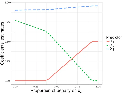
We demonstrate how the reduced–penalty procedure works using a toy example. A data set with n = 30 and p = 50 is simulated. We take the coefficient vector to be
β0 = (0.5 0.5 1 1 1 0 0 ...0)T and σ2 is taken to be one. The predictors are independent normal variables with the exception of 0.8 correlation between X(1) and X(2). Predictor 1 is included in the lasso model, however predictor 2 is not. Figure 1 presents the coefficients’ estimates of X(1), X(2) and X(3) when lowering the penalty ofX(2). Note howX(2) enters the model for low enough penalty whileX(1) leaves the model for low enough penalty (on
X(2)).
We suggest to measure the importance of a predictorj ∈S+ by the highestδ such that
j ∈S+L(δ). On the other hand, the importance of a predictorj0 ∈SL can be measured by
0.00 0.25 0.50 0.75 1.00
0.00 0.25 0.50 0.75 1.00
Proportion of penalty on x2
Coefficients' estimates
Predictor
x1
x2
x3
Figure 1: Toy example: coefficients’ estimates for predictorsX(1), X(2) andX(3)when low-ering the lasso penalty forX(2) only. The rightmost point corresponds to a lasso procedure with equal penalties for all predictors
Let ∆ = (δ0< δ1< ... < δh) be a grid of [0,1], with δ0 = 0 andδh = 1. For eachδ∈∆,
we obtain ˆβ+L(δ). Define
i?j =
argmax
i
{i: ˆβL+j(δi)6= 0} j /∈SL
argmax
i
{i: ˆβL+j(δi) = 0} j∈SL
and if the argmax is over an empty set, definei?j = 0. We suggest to chooseγj as follows:
γj =
0 j∈Sout
δi?
j/2 j∈S+
1−δi?
j/2 j∈SL,
for all j∈ {1, ..., p}. This choice of γ has the following nice properties.
• A predictor j /∈SL with i?j = 0 is excluded from consideration.
• On the other hand, for a predictorj∈SL, ifi?j = 0 thanγj = 1, which is the maximal
possible value. Even when the penalty for other predictors is dramatically reduced, leading to their entrance to the model,j remains part of the solution and hence it is essential for prediction ofY.
• Since predictors inSLwere picked when equal penalties were assigned to all predictors,
• However, for two identical predictors, X(j) =X(j0) (or highly correlated predictors) such that j ∈SL and j0 ∈/ SL, we get a desirable result. By Proposition 2, we know
that Xj0 ∈ S+. Now, for δh−1 < 1 it is clear that j0 ∈ S+L(δh−1) and j /∈ SL+(δh−1). Therefore. i?j =i?j0 =h−1 hence ifδh−1 is taken to be close to one, thenγj 'γj0 '0.5
as one might want.
Proposition 2 concerns two correlated predictors. In practice, the covariance structure ofX
may be much more complicated. Therefore the question arises: can we say something more general on the elastic net in the presence of competing models? Apparently we can. Let
M1 andM2 be two models, that is, two sets of predictors, that possibly intersect. Assume that the elastic net solution chose all the predictors in M1. What can we say about the predictors inM2? Are there conditions onXM2,XM1 and Y such that all the predictors in
M2 are also chosen? If the answer is yes (and it is, as Theorem 3 states), it justifies our use of the elastic net to reveal more relevant predictors. In our case, the relevant predictors are the building blocks of models inG.
In order to reveal this property of the elastic net, we analyze ˆβEN, the solution of (3), when assuming all the predictors inM1have non-zero values. DenoteM(−)for (M1∪M2)c, the set of predictors that are not included inM1 orM2 and ˜X=XM(−) for the appropriate
submatrix of X. Let ˆβMEN
1 , ˆβ EN
M2 and ˆβ EN
M− be the coordinates of ˆβEN that correspond to
M1,M2 and (M1∪M2)c, respectively. Let ˜Y =Y −X˜βˆMEN− be the unexplained residual of
Y, after taking into account ˜X. Finally, we show that both M1 and M2 are chosen by the elastic net if the prediction of ˜Y using M1, namely XM1βˆ
EN
M1 , projected onto the subspace
spanned by the columns ofM2 is correlated enough with ˜Y. Formally,
Theorem 3 Define βˆEN as before. Let M1 and M2 be two models with the appropriate submatrices XM1 and XM2. Define X˜ and Y˜ as before. Define βˆ
EN
M1 and
ˆ
βMEN
2 as before.
Denote PM2 for the projection matrix onto the subspace spanned by the columns of XM2.
WLOG, assume |M2| ≤ |M1| and that all the coordinates of βˆMEN1 are different than zero. Finally, if
˜
YTPM2XM1βˆ EN
M1 > c1(λ1, λ2, XM1,Y ,˜ βˆ EN
M1 ), (12)
then all the coordinates of βˆENM
2 are different than zero.
A proof and a discussion on the technical aspects of condition (12) and the constant c1 are given in the appendix. Theorem 3 states that under a suitable condition, predictors belonging to at least one of two competing models are chosen by the elastic net. In our context, when we have a model M1 with a good prediction accuracy, i.e., XM1βˆ
EN M1 is
close to ˜Y, then predictors in any another model M2 which has similar prediction, that is
PM2XM1βˆ EN
M1 is also close to ˜Y, would be chosen by the elastic net. Hence, these predictors
are expected to have a positive value in γ, and our simulated annealing algorithm would pass through these models, provided the conditions in Theorem 1 are met. Therefore, these models are expected to appear in G.
4. Simulation Studies
their capability to describe the underlying population can be found by the algorithm. The second simulation study examines the out–of–sample prediction error of models included in the minimal class of models.
We present below a scenario in which, other then the model used to create the data, there are three more models, that are not nested within the underlying model, with population prediction error close to the underlying model. In practice, all of these four models are of interest.
We consider Y =Xβ0+,∼N(0, I) with βj0 equals to C forj = 1,2, ...,6 and zero forj >6. C is a constant chosen to get a desired signal to noise ratio (SNR)||Xβ0||2. The predictors inX are all i.i.d.N(0, I) with the exception of X(7) andX(8), which are defined by
X(7) = 2 3[X
(1)+X(2)] +ξ
1, ξ1∼Nn
0,1
9I
X(8) = 2 3[X
(3)+X(4)] +ξ
2, ξ2∼Nn
0,1
9I
where ξ1 and ξ2 are independent. In this scenario, there are 4 models we would like to find: (I) {1,2,3,4,5,6}; (II) {5,6,7,8}; (III) {3,4,5,6,7}; and (IV) {1,2,5,6,8}. In particular, each of these models minimizes the population prediction errorE||Y −XSβS||22}for models with its size. That is, Model (I) minimizes the population prediction error for models of size k = 6, Model (II) minimizes the prediction error for models of size k = 4, and both models (III) and (IV) minimize the prediction error for models of sizek= 5. Furthermore, it can be shown, for example, that the population prediction error of Model (III) is just 3.7% larger than the error of true model for SN R = 1, 14.8% for SN R = 2, and larger values for SN R≥4
Note that while models (II)–(IV) do not describe the data as well as Model (I), they contain less predictors. Furthermore, in an hypothetical real-life situation where future measurements were to be made on the predictors and the outcome, and, for the sake of the example, X(1) or X(2) were more expensive to measure, models (II)–(IV) could have provided a frugal alternative, while preserving a reasonable prediction error.
As part of this simulation study, for each simulated data set, we do the following:
1. Obtain γ as explained in Section 3.2. The tuning parameter of the lasso is taken to be the minimizer of the cross–validation MSE. For the elastic net,αin (4) is taken to be 0.4.
2. Run the simulated annealing algorithm for κ = 4,5,6. The tuning parameters of the algorithm are chosen quite arbitrarily: T = (10×0.71,10×0.72, ...,10×0.720); ∆ = (0,0.02,0.04, ...,0.98,1); Nt=N = 100 for allt∈T.
p= 200 p= 500 p= 1000 SNR Model Best Top 5 Best Top 5 Best Top 5
1
(I) 0.00 0.01 0.00 0.00 0.00 0.00 (II) 0.42 0.62 0.28 0.46 0.23 0.38 (III) 0.04 0.08 0.01 0.02 0.00 0.00 (IV) 0.04 0.08 0.02 0.03 0.00 0.01
2
(I) 0.10 0.12 0.05 0.06 0.04 0.05 (II) 0.94 0.96 0.92 0.94 0.94 0.95 (III) 0.27 0.34 0.18 0.24 0.15 0.17 (IV) 0.28 0.37 0.18 0.22 0.14 0.17
4
(I) 0.38 0.38 0.20 0.20 0.11 0.11 (II) 0.96 0.96 0.96 0.96 0.96 0.95 (III) 0.38 0.46 0.31 0.36 0.22 0.24 (IV) 0.39 0.46 0.28 0.31 0.24 0.26
8
(I) 0.72 0.72 0.46 0.46 0.32 0.32 (II) 0.97 0.97 0.97 0.97 0.96 0.96 (III) 0.41 0.48 0.36 0.40 0.30 0.31 (IV) 0.44 0.50 0.34 0.37 0.29 0.31
12
(I) 0.86 0.86 0.66 0.66 0.49 0.49 (II) 0.98 0.98 0.97 0.97 0.96 0.96 (III) 0.49 0.55 0.41 0.44 0.32 0.34 (IV) 0.42 0.48 0.37 0.40 0.32 0.34
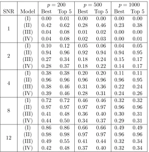
Table 1: Proportion that each model is chosen as best model or as one of top five models for different number of potential predictors (p) and various SNR values.
A 1000 simulated data sets were generated for each different scenario: For n = 100, p = 200,500,1000 and for SNR = 1,2,4,8,12,16. Table 1 displays the proportion of times each model was chosen, either as the best one, or as one of the top five models. The results are as one might expect. For large SNR, the models are chosen more frequently. However, models (III) and (IV) are competing, in the sense that they both include five predictors. Even for large SNR, each of the models, (III) and (IV), is chosen in about 50% of the cases. Therefore, as recommended in Section 3.1, we repeat the simulations while starting the algorithm from different initial points, that is, different initial models.
Figure 2 presents comparison between running the algorithm from one and three starting points. When we initiated the algorithm from three different models, the results improved for all models, and in particular for models (III) and (IV). The results described in this section are quite similar to the results we obtained when formingG(κ, η) as defined in (6), for each κ= 4,5,6 separately and using arbitrary small values ofη.
p = 200 p = 500 p = 1000
0.00 0.25 0.50 0.75 1.00
4 8 12 16 4 8 12 16 4 8 12 16
SNR
Pr
opor
tion that a model was c
hosen
Starting points
One Three
Model
(I) (II) (III) (IV)
Figure 2: Proportion that each model is chosen as one of top five models for different number of potential predictors (p) and various SNR values. There is an apparent improvement when running the algorithm from three starting points.
β0 is created in the same as in Scenario 1, but a more complex correlation structure is considered for X. First, define Σ(m) to be an m×m covariance matrix defined so for all i = 1, ..., m and j = 1, , ., m, Σij(m) = 0.75|i−j|. The subvector containing the first 5 predictors, (X(1), X(2), ..., X(5)) is created with the covariance matrix Σ(5). Then, each of the next 10 predictors X(j), j = 6,7...,15 is correlated with two predictors that are not part of the true model. For example, (X(6), X(21), X(22)) is simulated from N3(0,Σ(3)) and (X(7), X(23), X(24)) is simulated from N3(0,Σ(3)). The remaining predictors are simulated as iid N(0,1). In Scenario 3,X is created as in Scenario 2, but the coefficients in the true model are now all equal. That is, βj0 =C, j = 1,2, ...,20, with C being a constant chosen to get a desired SNR.
Scenario 1 Scenario 2 Scenario 3
1 2 3
1 2 3
1 2 3
p = 200
p = 500
p = 1000
2 4 6 8 2 4 6 8 2 4 6 8
SNR
Out−of−sample prediction relative to the lasso
Method
Avg (size=15) Avg (size=20) Avg (size=25) Min (size=15) Min (size=20) Min (size=25) Elastic net Lasso Adaptive lasso
Figure 3: Out–of–sample prediction error for different scenarios, different number of poten-tial predictors (p) and various SNR values. Methods compared are lasso, elastic net and adaptive lasso, as well as the average (avg) and minimal (min) error in the minimal class of models, with model size of 15,20 and 25 predictors. The classes were built by combining 5 best models obtained from three runs of the simulated annealing search algorithm.
relative to the out–of–sample prediction error of the lasso. For SNR=1, the lasso performs the best, for all three scenarios considered, although the other methods show comparable performance. Under Scenarios 1 and 2, when the non–zero parameters are created from a normal distribution, so some predictors are stronger and others are weaker, the best model identified by the minimal class, for either κ = 20 or κ = 25, outperforms other methods for SNR>1. Under Scenario 3, where all coefficients (in the true model) are equal, the same pattern is observed for SNR>4. For large SNR values, under Scenario 3, the models in the minimal class of size 15 are underperforming. While under Scenarios 1 and 2, the predictors missed by the minimal class withκ= 15 are likely to be those with small effect, under Scenario 3 all predictors have an equal effect. We also considered scenarios with X
simulated from Np(0,Σ(p)). The results are similar to those observed for Scenario 1 and
hence are omitted.
5. Real data sets
0 10 20 30 40
0.00 0.25 0.50 0.75 1.00 γ
count
(a) Riboflavin data
0 10 20 30
0.00 0.25 0.50 0.75 1.00 γ
count
(b) Air pollution data
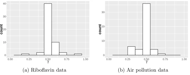
Figure 4: Histograms of the values ofγ for positive entries only in the two data set analysis examples.
T = 10×(0.71,0.72, ...,0.720), ∆ = (0,0.01,0.02, ...,0.98,0.99,1), and Nt=N = 100 for all t∈T.
5.1 Riboflavin
We use a high–dimensional data about the production of riboflavin (vitamin B2) in Bacillus subtilis that were recently published (B¨uhlmann et al., 2014). The data consist p = 4088 predictors. These are measures of log expression levels of genes inn= 71 observations. The target variable is the (log) riboflavin production rate.
The lasso model SL includes 40 predictors (and intercept), and the elastic net model SEN includes 59 predictors. In total, we get 61 different predictors (i.e., genes). Panel (a)
of Figure 4 presents the histogram of the positive values inγ.
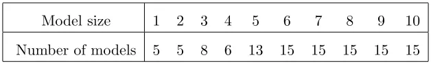
We run the algorithm from three random starting points for each model size between 1 and 10. We keep the five best models for each size and starting point, to get, after removal of duplicates, a total of 112 models. See Table 2 for the number of unique models as a function of the model size. Following a referee comment, we note here that in practice models with low model size may have unacceptably low R2, and this can be checked in practice. In our analysis here we keep these models since the R2 values are all larger than 0.35 and to ease the exposition, so we would be able to compare the search results to models obtained by other methods. The models found by other methods, for the riboflavin data, are of a relatively small size; see B¨uhlmann et al. (2014)
The following insights are drawn from examining more carefully the models we obtained (see Table 1 in the online appendix):
• In total, the models include 53 different predictors. Out of these, 35 predictors appear in less than 10% of the models, meaning they are probably less important as predictors of riboflavin production rate.
Model size 1 2 3 4 5 6 7 8 9 10
Number of models 5 5 8 6 13 15 15 15 15 15
Table 2: Riboflavin data: Number of unique models for each model size after running the algorithm from 3 different starting points
this gene does not hold an effect strong enough comparing to other genes in order to stand out, it has a unique relation with the outcome predictor that could not be mimicked using other combination of genes.
• At least one gene from the group {4002,4003,4004,4006} is contained in all models of size larger than one, although never more than one of these genes. Genes number 4003 and 4004 appear more frequently than genes number 4002 and 4006. Looking at the correlation matrix of these genes only, we see they are all highly correlated (pairwise correlations > 0.97). Future research could take this finding into account by using, e.g., the group lasso (Yuan and Lin, 2006).
• Similarly, either gene number 1278 or gene number 1279 appear in about half of the models. They are also strongly correlated (0.984). The same statement holds for genes number 69 and 73 (correlation of 0.945) as well.
• The importance of genes number 792,1131, and possibly others, should be also exam-ined since each of them appears in a variety of different models.
We now compare our results to models obtained using other methods, as reported in B¨uhlmann et al. (2014). The multiple sample splitting method to get p–values (Mein-shausen et al., 2009) yields only one significant predictor. Indeed, a model that includes only this predictor is part of our models. If one constructs his model using the stability selection (Meinshausen and B¨uhlmann, 2010) as a screening process for the predictors, he would get a model consisting three genes, which correspond to columns number 625,2565 and 4004 in our X matrix. However, this model is not included in our top models. In fact, the highest MSE for a model in our 8 models of size 3 is 0.2047 while the MSE of the model suggested using the stability selection is 0.2703, more than 30% difference!
5.2 Air pollution
We now demonstrate how the proposed procedure can be used for traditional, purportedly simpler, problem. The air pollution data set (McDonald and Schwing, 1973) includes 58 Standard Metropolitan Statistical Areas (SMSAs) of the US (after removal of outliers). The outcome variable is age-adjusted mortality rate. There are 15 potential predictors including air pollution, environmental, demographic and socioeconomic predictors. Description of the predictors is given in Table 4 in the appendix.
variable, namely natural logarithm, square root and power of two transformations. Consid-ering also all possible two way interactions, we have a total of 165 predictors.
High–dimensional regression model that includes transformations and interactions has been dealt with in the literature. For example, by using two step procedures (Bickel et al., 2010) or by solving a relevant optimization problem (Bien et al., 2013). Our procedure has a different goal, since we are not looking for the best predictive model, but rather for meaningful insights about the data.
Following the lasso and elastic net step, we are left with 51 predictors with positive γj
(6 untransformed predictors, 4 log transformations, 6 square root transformations, 9 power of two transformations and the rest are interactions). Panel (b) of Figure 4 presents the histogram of the positive values in γ.
We modify the search algorithm to make it produce results typical to an analysis in-volving interaction terms. In particular, we search for models such that an interaction term is included only if at least one of the corresponding main terms is included in the model. In order to do so, the definitions in (7) and (8) are modified such that the probability of proposing an interaction term is zero if none of the corresponding main effects is in this model (excluding the variable chosen to be taken out). On the other hand, main effects are “protected” of being suggested to be excluded from the model, if any interaction involving them is part of the current model. We achieve this by setting to zero the probability of suggesting a predictor when an interaction term involving this predictor is included.
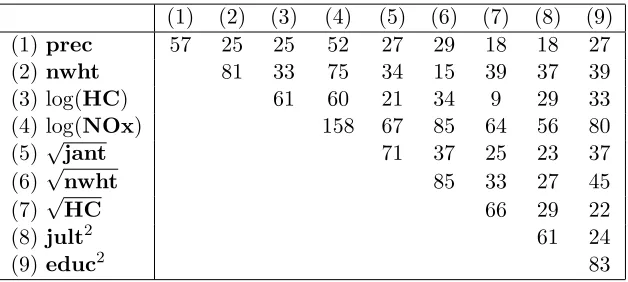
Following our earlier comment on considering satisfactory models, and since we are looking for more complex models in this example, considering the option of transformations and interactions, we run the algorithm for κ = 5,6, ...,15, for each κ, from three starting points, and then we keep the 5 best models. In total, we get 164 unique models. Table 3 summarizes the results for prominent main effect predictors, that is, predictors that appear in at least third of the models we obtained. The table presents a matrix of the joint frequency of each two predictors. Each cell in the table is the number of models including both the predictor listed in the row and the predictor listed in the column. The diagonal is simply the number of models that a predictor appears in. Considering Table 3, the nitric oxide pollution is invaluable for prediction of mortality rate. This predictor (in a log shape) appears in a large majority of the models. The percentage of non–white population also appears in most models. In almost half of them, it appears untransformed, but the same could be said about this predictor after square root transformation. However, in less than 10% of the models, this predictor appears in both forms. We conclude that this predictor should be used for prediction of the mortality rate, but the question of transformation remains unsolved. Similar comments can be made about hydrocarbon pollution.
(1) (2) (3) (4) (5) (6) (7) (8) (9)
(1)prec 57 25 25 52 27 29 18 18 27
(2)nwht 81 33 75 34 15 39 37 39
(3) log(HC) 61 60 21 34 9 29 33
(4) log(NOx) 158 67 85 64 56 80
(5)√jant 71 37 25 23 37
(6)√nwht 85 33 27 45
(7)√HC 66 29 22
(8)jult2 61 24
(9)educ2 83
Table 3: Frequency that each two predictors together in the 164 models. The diagonal is simply the number of models that a predictor appears in. For example, in 67 models both log(NOx) and √jant appear.
preliminary steps. However, the absence of age related effect is not so surprising since the outcome variable, the mortality rate, is age corrected. Nevertheless, since the interaction term appeared in about half of the models that included January temperature as a predictor, it can be considered if the main effect is also considered.
6. Discussion
Model selection consistency is an ambitious goal to achieve when dealing with high–dimensional data. A “minimal class of models” was defined to be a set of models that should be con-sidered as candidates for prediction of the outcome variable. A search algorithm to identify these models was developed using a simulated annealing method. Under suitable conditions, that are outlined in Theorem 1, the algorithm passes through models of interest.
A score for each predictor is given using the lasso, the elastic net and a reduced–penalty lasso. These scores are used by the search algorithm. They are not necessarily optimal but we claim that they are sensible. Other scoring methods may achieve better results. On the other hand, the scores we use here may be used for other purposes. Theoretical justification for using the elastic net to unveil predictors the lasso might have missed was also presented. A simulation study demonstrated the capability of the search algorithm to detect relevant models.
One possible limitation of the proposed algorithm is the number of tuning parameters to be chosen. In our simulation studies and data analyses, we have found the algorithm to be quite robust to the parameters’ specification. For ease of applications, we now list suggested default values for some of the parameters. The tuning parameter of the lasso λ, can be chosen by cross validation. Since the subsequent use of the elastic net is to bring into surface potential predictors, relatively low value forαin (4) can be taken, sayα∈(0.2,0.5). A possible choice for ∆ is (0,0.01,0.02, ...,1). As always when using simulated annealing,T
and Ntmay be more complicated to choose. We used for all simulations and data analyses
the sequenceT = (10×0.71,10×0.72, ...,10×0.720) andNt= 100. This leaves us with the
and, for example, comparing the MSEs for κ = 5 and κ = 10, may imply if there is a substantial benefit when adding variables, before moving to larger models. Similarly to many algorithms, the proposed simulated annealing algorithm should be initiated from multiple points.
As illustrated using real data examples, a class of minimal models can be used to derive conclusions regarding the problem at hand. This is rarely the case that a researcher believes a one true model exists, especially in the p > nregime. Therefore, we suggest to abandon the search for this “holy grail”, and to analyze the class of minimal models instead. While retreating from the choice of a single model, and instead analyzing group of models, offers advantages, it may complicate standard data analysis in at least two ways, even when putting computational issues aside. The first is a practical one and concerns the question of which analyses should be carried out once a minimal class of models, or at least its sample version, is obtained. Model averaging can be used to estimate association parameters. Similarly, predictions from multiple models can be averaged. More precise predictions or estimates may be obtained by coupling the obtained models with weights, possibly using the empirical MSEs. More robust aggregation can be obtained by using medians instead of averages, to deal with the fact that each model consists of a different number of predictors. Another, less formal, data analysis strategy is to combine subject matter knowledge with wealth of many models. We have demonstrated such exploratory analyses in Section 5, by comparing the proportion of models each predictor, or multiple predictors, are included.
The second issue is a conceptual one. If we indeed quit from searching for a single model, i.e., a single group of predictors, what are our assumptions about the underlying mechanism that the data came from. Do we believe such a mechanism exists? One answer is that we do not need to think about how the data was created, but how can we describe the data. This, however, offers only a partial answer because we are focused on exploratory analysis, while model selection is of interest from inferential perspective as well. If more than one model describes the data adequately, which one is the true one? Does it matter? While most data are not created following one’s computer program, disbelieving in the existence of a true model certainly gives rise to further questions.
It is well known that achieving good prediction and successful model selection simulta-neously, in a reasonable computation time, is impossible, especially in the high–dimensional setting. We therefore suggested here to make a compromise. Our approach is not neces-sarily optimal for prediction, nor for model selection. However, it offers a data analysis method that takes into account the uncertainty in model selection, but ensures reasonable prediction accuracy. This method can be used for either prediction, parameter estimation or model selection.
Acknowledgments
We thank two anonymous reviewers for useful comments and suggestions that improved the paper. This research was supported by ISF grant 1770/15
Appendix A. Proofs
A.1 Proof of Theorem 1
We start with the following lemma.
Lemma 4 Assume Y = µ+ and assume also (A1)–(A4). Let Sk = {S :|S|= k,βˆS =
(XSTXS)−1XSTY} be the set of all models with k variables, such that βˆS, the LS estimate,
is unique. Denote Sj? =S∪ {j}, j /∈S for a model that includes S and additional variable
j not inS. We have
max
S∈Sk
1≤j≤p
T(XS? j
ˆ
βS? j −XS
ˆ
βS) =op(n)
Letξj be the vector of coefficients obtained by regressing X(j), thejthcolumn in X, onXS
and let Pj be the projection operator on the subspace spanned by the part ofX(j) which
is orthogonal to the subspace spanned byXS. That is,
Pj =
(X(j)−XSξj)(X(j)−XSξj)T ||X(j)−X
Sξj||22
.
Let ˆβSj?
j be the coefficient estimate of X
(j) in model S?
j, and let ˆβ
−j S?
j be the coefficient
estimates of the variables inS but for the modelSj?. Since (X(j)−XSξj) is orthogonal to
the subspace spanned by the columns of XS we have
XS? j
ˆ
βS? j =X
(j)βˆj S?
j +XS
ˆ
βS−?j j
= (X(j)−XSξj) ˆβSj?
j +XS( ˆβ
−j S?
j +ξj
ˆ
βjS? j)
= (X(j)−XSξj) ˆβSj? j +XS
ˆ
βS
=Pjy+XSβˆS.
Therefore,
T(XS? j
ˆ
βS? j −XS
ˆ
βS) =TPjµ+TPj.
Now, since ||Pjµ||22 ≤ ||µ||22 = O(n), we get that for all j, TPjµ = Op( √
n). Next, let
Z1, ..., Zpk+1 beN(0, σ2) random variables and observe that the approximate size of the set {Sk} × {1, ..., p}is pk+1. We have for any a >0
P
max S∈Sk
1≤j≤p
1
n TP
j≥a
≤P
max
1≤j≤pk+1|Zj| ≥
r an σ2 ≤σ r
2(k+ 1) logp+o(1)
an .
Now, since p=nα and k=o(n/logn) we get that
P
max S∈Sk
1≤j≤p
1
n TP
j≥a
=o(1)
We can now move to the proof of Theorem 1. For simplicity, the notation of i as the iteration number for the current temperature t is suppressed. Note that it is enough to only consider models such that S∩S¯ =∅ and to consider m =s0. Denote Qt(S, g, j) for
the probability of a move in the direction of ¯S in the next iteration, that is, the probability of choosing a variable j ∈ S ∩S¯c and replace it with a variable g ∈ Sc∩S¯. Denote
S0 ={S/{j}} ∪ {g} for this new model. We have
Qt(S, g, j)
=P r(S→S0) min
"
1,exp ||Y −XS ˆ
βS||22− ||Y −XS0βˆS0||2
2
t
!
P r(S0 →S)
P r(S →S0)
#
(13)
whereP r(S→S0) is the probability of suggestingS0, given current model isS. Now, since
γmin ≥ cγ and since the maximal value in γ equals to one by definition, we have for all S ⊆Aγ,
cγ(hγ−s0)≤
X
u /∈S
γu≤hγ−s0
s0 ≤
X
v∈S
1
γv ≤ s0
cγ
. (14)
Now, by substituting (14) into (7)–(9) we get
P r(S →S0) = P γg u /∈Sγu
1/γj P
v∈S γ1v
≥ c
2
γ s0(hγ−s0)
,
P r(S0 →S)
P r(S →S0) =
γj2 γ2
g P
u /∈Sγu P
v∈S
1
γv
P
u /∈S0γuPv∈S0 γ1
v
≥c4γ.
(15)
Next, we have
1
n||Y −XS
ˆ
βS||22− 1
n||Y −XS0
ˆ
βS0||22
= 1
n h
(Y −XS0βˆS0) + (Y −XSβˆS)
iT
XS0βˆS0−XSβˆS
= 1
nY
TX
S0βˆS0 −XSβˆS
= 1
nµ
T X
S0βˆS0 −XSβˆS
+ 1
n
T X
S0βˆS0−XSβˆS
= 1
nµ
T X
S0βˆS0 −XSβˆS
+ ∆n(S, S0) (16)
where the second equality is due to ˆβS and ˆβS0 being LS estimators. We get that an
estimator in linear model achieves better (lower) sample MSE, if the correlation of the prediction using this estimator withY is larger. Now, denote S00=S0∪S. We have
∆n(S, S0) =
1
n T h(X
S00βˆS00−XSβˆS)−(XS00βˆS00−XS0βˆS0)
and if we apply Lemma 4 twice we get that ∆n(S, S0) = op(1). Now, regarding the first
term in (16),
1
nµ
T X
S0βˆS0−XSβˆS
= 1
nµ T(P
S0y− PSy)
= 1
n ||PS0µ||
2
2− ||PSµ||22
+ ∆0n(S, S0)
(17)
where ∆0n(S, S0) = 1nµT [PS0− PS]. The content of the proof of Lemma 4 implies that
∆0n(S, S0) =op(1). Now, by (16) and (17) and since Assumption (B1) holds for t0 we get that for large enough n
1
n
||Y −XSβˆS||22− ||Y −XS0βˆS0||22
≥4tlogcγ. (18)
Now, by substituting (15) and (18) into (13) we get that for large enough n,
Qt0(S, g, j)≥
c2γ s0(hγ−s0)
for allS 6= ¯S,j ∈S∩S¯c and g∈Sc∩S¯. (11) follows from this immediately since for any integerm and for all S6= ¯S,
Ptm0(S0|S)≥ min {S:S∩S¯=∅}
j∈S∩S¯c g∈Sc∩S¯
[Qt(S, g, j)]s0 ≥ "
c2γ s0(hγ−s0)
#s0
.
A.2 Proof of Proposition 2
Recall that the elastic net estimator ˆβEN minimizes
||Y −Xβ||22+λ1|β|+λ2||β||22 (19)
Now, WLOG assume that ˆβEN is a solution such that ˆβ1EN >0. For convenience, we omit the “EN” superscript from now on (i.e., ˆβ = ˆβEN). Define the subspace
B:={β :∀i= 16 ,2 βi = ˆβi, β1 =τβˆ1, β2= (1−τ) ˆβ1}. (20) If the minimum of (19) over B is obtained for τ 6= 1, then given that X(1) is part of the elastic net model, predictor X(2) is also part of this model.
WLOG, write down X as X = (X(12) X−(12)) where X(12) = (X(1) X(2)) are the first two columns of X and X−(12) are the rest of its columns. Similarly, we have βT = (βT(12) βT−(12)) where β(12) is the first two entries in the vectorβ and β−(12) is the rest of the vector. Define ˜Y =Y −X−(12)β−(12). We can rewrite (19) as
||Y˜ −X(12)β(12)||2
2+λ1(|β−(12)|+|β(12)|) +λ2(||β−(12)||22+||β(12)||22) (21) If the minimum of (21), on B, is achieved at 0 < τ∗ < 1 then ˆβ2 must be non zero. Minimizing (21) onB is essentially minimizing
onB . Now, by the definition ofBin (20) and using simple algebra we get that (22) equals to
2
ˆ
β1Y˜T
τ(X(2)−X(1))−X(2)−βˆ12τ(1−τ)(1−ρ) +λ2βˆ12
1
2−τ(1−τ)
.
This is a quadratic function ofτ, and by equating its derivative to zero we get that
τ∗= 1 2 −
˜
YT(X(2)−X(1)) 2 ˆβ1(λ2+ 1−ρ)
is the minimizer of (19) (the coefficient of the quadratic term is positive). Note that for
X(2)=X(1) we get the expectedτ∗ = 1
2 solution. Note also that this reveals no information regarding the lasso where λ2 = 0. Next, we get that 0< τ∗ <1 if
˜
YT(X(2)−X(1)) ˆ
β1(λ2+ 1−ρ)
<1. (23)
Since ||X(2)−X(1)||2
2= 2(1−ρ) we have
|Y˜T(X(2)−X(1))| ≤ n X
i=1
|Y˜i||Xi(2)−X
(1)
i | ≤ ||Y˜||2
p
2(1−ρ),
using the triangle inequality and then Cauchy–Schwartz inequality. It is assumed that ˆ
β1 ≥cβ >0 and it is known that||Y˜||2 ≤ ||Y||2. Therefore, we may rewrite (23) as
√
2||Y||2√1−ρ cβ(λ2+ 1−ρ)
<1.
Now, Denotet=√1−ρ, u= ||Y||2
cβ , we have
t2−√2ut+λ2 >0.
Forλ2 > 12u2, we get the result we want for allρ’s. Forλ2 < u
2
2 we have
p
1−ρ > √1
2(u+
p
u2−2λ
2), (24)
p
1−ρ < √1
2(u−
p
u2−2λ
2). (25)
The RHS of (24) is larger than 1 if λ2 <
√
2u−1. That is, there is no suitable ρ for this case. The RHS of (25) is always positive, and for the same condition λ2 <
√
2u−1, it also meaningful, i.e., (u−√u2−2λ
2)<
√
2 and in terms of ρ,
ρ >1−1
2(u−
p
u2−2λ 2)2 or alternatively,
ρ >1− u
2 2 1−
r
1−2λ2
and by Taylor expansion for 2λ2/uwe get
ρ >1− λ
2 2 2u2
A.3 Proof of Theorem 3
The proof is similar to the proof of Proposition 2. Let ˆβ = ˆβEN be the elastic net estimator and denote ˆβM for the values in ˆβ corresponding to the set of predictors M. We can
partition the set of potential predictors{1,2, ..., p}to four disjoint subsets: M(−);M1∩M2c;
M1c∩M2 andM1∩M2. We replace (20) with
B:={β :βM(−) = ˆβM(−) βM1∩M2 = ˆβM1∩M2, (26)
βM1∩M2c =τ
ˆ
βM1∩M2c, βM1c∩M2 = (1−τ)Θ
0βˆ
M1∩M2c}. (27)
whereβM is defined as the values in ˆβ corresponding to the set M and Θ0 is the matrix of
coefficients obtained from regressingXM1∩M2c onXM1c∩M2. We define Θ to be an augmented
version of Θ0, which we obtain by regressingXM1 onXM2. That is,
XM2Θ =PM2XM1 (28)
Note that on B,
Xβ = ˜XβˆM(−)+τ XM1βˆM1+ (1−τ)XM2Θ ˆβM1
Recalling that ˜Y =Y −X˜βˆM(−), minimizing (3) on B is equivalent to minimize
||Y˜ −τ XM1βˆM1 −(1−τ)XM2Θ ˆβM1||
2
2+λ1[τ||βˆM1||1+ (1−τ)||Θ ˆβM1||1]
+λ2[τ2||βˆM1||
2
2+ (1−τ)2||Θ ˆβM1||
2
2] (29) as a function ofτ. Using a first–order condition and substituting (28) we find that (29) is minimized for
τ∗ =
−( ˜Y − PM2XM1βˆM1)
T(I− P
M2)XM1βˆM1 + λ1
2(||βˆM1||1− ||Θ ˆβM1||1)−λ2||Θ ˆβM1||
2 2
||(I− PM2)XM1βˆM1||
2
2−λ2||βˆM1||
2
2−λ2||Θ ˆβM1||
2 2
. (30)
Before we continue, note that ifX2 =X1then Θ is the identity matrix and PM2XM1 =X1.
Substituting these facts into (30), we get that τ∗ = 12 as one might expect. Same result is obtained for the caseM2 ⊆M1.
As it can be seen in (26), the coordinates of ˆβM2 are all different than zero if τ
∗ <1.
Now, since PM2(I− PM2) = 0 we get thatτ∗<1 if
−Y˜T(I− PM2)XM1βˆM1 +||(I− PM2)XM1βˆM1||
2 2−
λ1
2 ||Θ ˆβM1||1
>−λ1
2 ||βˆM1||1−λ2||βˆM1||
2 2 which is certainly true if
˜
YTPM2XM1βˆM1−
λ1
2 ||Θ ˆβM1||1 >−
λ1
2 ||βˆM1||1−λ2||βˆM1||
2
2+ ˜YTXM1βˆM1 (31)
Appendix B. Supplementary table for Section 5.2
Predictor Description
prec Mean annual precipitation in inches jant Mean January temperature in degrees F jult Mean July temperature in degrees F age65 Percentage of population aged 65 or older pphs Population per household
educ Median school years completed by those over 22
h facl Percentage of housing units which are sound and with all facilities dens Population per square mile in urbanized areas
nwht Percentage of non–white population in urbanized areas wtcl Percentage of employed in white collar occupations
linc Percentage of families with income<3,000 dollars in urbanized areas
HC Relative pollution potential of hydrocarbon NOx Relative pollution potential of nitric oxides SUL Relative pollution potential of sulfur dioxide
hum Annual average percentage of relative humidity at 1pm
Table 4: Potential predictors for mortality rate in Section 5.2
References
Hirotugu Akaike. A new look at the statistical model identification. IEEE transactions on automatic control, 19(6):716–723, 1974.
Peter J Bickel and Mu Cai. Discussion of Sara van de Geer: Generic chaining and the `1 penalty. Journal of Statistical Planning and Inference, 143(6):1013–1018, 2012.
Peter J Bickel, Yaacov Ritov, and Alexandre B Tsybakov. Simultaneous analysis of lasso and dantzig selector. Annals of Statistics, 37(4):1705–1732, 2009.
Peter J Bickel, Yaacov Ritov, and Alexandre B Tsybakov. Hierarchical selection of vari-ables in sparse high-dimensional regression. In Borrowing strength: theory powering applications–a Festschrift for Lawrence D. Brown, volume 6, pages 56–69. Institute of Mathematical Statistics, 2010.
Jacob Bien, Jonathan Taylor, and Robert Tibshirani. A lasso for hierarchical interactions. Annals of Statistics, 41(3):1111–1141, 2013.
Leo Breiman. Bagging predictors. Machine Learning, 24(2):123–140, 1996.
S. P. Brooks, N Friel, and R King. Classical model selection via simulated annealing.Journal of the Royal Statistical Society: Series B (Statistical Methodology), 65(2):503–520, 2003.
Peter B¨uhlmann, Markus Kalisch, and Lukas Meier. High-dimensional statistics with a view toward applications in biology. Annual Review of Statistics and Its Application, 1: 255–278, 2014.
Florentina Bunea, AlexandreB. Tsybakov, and MartenH. Wegkamp. Aggregation and Sparsity Via `1 Penalized Least Squares. In Learning Theory, volume 4005 of Lecture Notes in Computer Science, pages 379–391. Springer Berlin Heidelberg, 2006. URL
http://dx.doi.org/10.1007/11776420_29.
Florentina Bunea, Alexandre Tsybakov, and Marten Wegkamp. Sparsity oracle inequalities for the lasso. Electronic Journal of Statistics, 1:169–194, 2007.
Jerome Friedman, Trevor Hastie, and Rob Tibshirani. Regularization paths for generalized linear models via coordinate descent. Journal of statistical software, 33(1):1–22, 2010.
Eitan Greenshtein and Ya’Acov Ritov. Persistence in high-dimensional linear predictor selection and the virtue of overparametrization. Bernoulli, 10(6):971–988, 2004.
W Keith Hastings. Monte Carlo sampling methods using Markov chains and their applica-tions. Biometrika, 57(1):97–109, 1970.
Nils Lid Hjort and Gerda Claeskens. Frequentist model average estimators. Journal of the American Statistical Association, 98(464):879–899, 2003.
Arthur E Hoerl and Robert W Kennard. Ridge regression: Biased estimation for nonorthog-onal problems. Technometrics, 12(1):55–67, 1970.
Jennifer A Hoeting, David Madigan, Adrian E Raftery, and Chris T Volinsky. Bayesian model averaging: A tutorial. Statistical Science, pages 382–401, 1999.
Jian Huang, Shuangge Ma, and Cun-Hui Zhang. Adaptive lasso for sparse high-dimensional regression models. Statistica Sinica, 18(4):1603, 2008.
Jinzhu Jia and Bin Yu. On model selection consistency of the Elastic Net when p >> n. Statistica Sinica, 20:595–611, 2010.
Scott Kirkpatrick, D. Jr. Gelatt, and Mario P Vecchi. Optimization by simulated annealing. science, 220(4598):671–680, 1983.
Gary C McDonald and Richard C Schwing. Instabilities of regression estimates relating air pollution to mortality. Technometrics, 15(3):463–481, 1973.
Nicolai Meinshausen and Peter B¨uhlmann. High-dimensional graphs and variable selection with the lasso. Annals of Statistics, 34(3):1436–1462, 2006.