Communication-Optimal Distributed Dynamic Graph Clustering

(1)

The Thirty-Third AAAI Conference on Artificial Intelligence (AAAI-19)

Communication-Optimal Distributed Dynamic Graph Clustering

Chun Jiang Zhu,

1

_{Tan Zhu,}

1

_{Kam-Yiu Lam,}

2

_{Song Han,}

1

_{Jinbo Bi}

1 1_{Department of Computer Science and Engineering, University of Connecticut, Storrs, CT, USA}

{chunjiang.zhu, tan.zhu, song.han, jinbo.bi}@uconn.edu

2_{Department of Computer Science, City University of Hong Kong, Hong Kong, PRC} [email protected]

Abstract

We consider the problem of clustering graph nodes over large-scale dynamic graphs, such as citation networks, im-ages and web networks, when graph updates such as node/edge insertions/deletions are observed distributively. We propose communication-efficient algorithms for two well-established communication models namely the message passing and the blackboard models. Given a graph withn

nodes that is observed atsremote sites over time[1, t], the two proposed algorithms have communication costsO˜(ns)

and O˜(n +s) (O˜ hides a polylogarithmic factor), almost matching their lower bounds,Ω(ns)andΩ(n+s), respec-tively, in the message passing and the blackboard models. More importantly, we prove that at each time point in[1, t]

our algorithms generate clustering quality nearly as good as that of centralizing all updates up to that time and then ap-plying a standard centralized clustering algorithm. We con-ducted extensive experiments on both synthetic and real-life datasets which confirmed the communication efficiency of our approach over baseline algorithms while achieving com-parable clustering results.

1 Introduction

Graph clustering is one of the most fundamental tasks in artificial intelligence and machine learning (Giatsidis et al. 2014; Tian et al. 2014; Anagnostopoulos et al. 2016). Given a graph consisting of a node set and an edge set, graph clustering asks to partition graph nodes into clus-ters such that nodes within the same cluster are “densely-connected” by graph edges, while nodes in different clus-ters are “loosely-connected”. Graph clustering on modern large-scale graphs imposes high computational and storage requirements, which are too expensive, if not impossible, to obtain from a single machine. In contrast, distributed com-puting clusters and server storages are a popular and cheap way to meet the requirements. Distributed graph clustering has received considerable research interests (Hui et al. 2007; Yang and Xu 2015; Chen et al. 2016; Sun and Zanetti 2017). However, the dynamic nature of modern graphs makes the clustering problem even more challenging. We discuss sev-eral motivational examples and their characteristics as fol-lows.

time point :τ time point :

τ + 1

Coordinator

:

τ

:

τ + 1

:

τ τ:

:

τ + 1 τ + 1:

S1 S2 S3

Communication

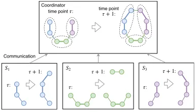
Figure 1: Illustration of distributed dynamic graph cluster-ing. Thick edges have an edge weight 3 while thin edges have an edge weight 1. Clustering results are evolving over time.

Citation Networks.Graph clustering on citation networks aims to generate groups of papers/manuscripts/patents with many similar citations. This implies that the authors within each cluster share similar research interests. The clustering results can be useful for recommending research collabo-ration, e.g. in ResearchGate. Large-scale citation networks, e.g. the US patent citation network (1963-1999)1_{, contain} millions of patents and tens of millions of citations, and they are dynamic with frequent insertions. New papers are pub-lished everyday with new citations to be added to the net-work graph. Citation netnet-works usually have negligible dele-tions because very few works get revoked.

Large Images.Image segmentation is a fundamental task in computer vision (Arbelaez et al. 2011). Graph-based image segmentation has been studied extensively (Shi and Malik 2000; Maier, Luxburg, and Hein 2009; Kim et al. 2011). In these methods, each pixel is mapped into a node in a high-dimensional space (considering coordinates and inten-sity) that then connects to its K-nearest nodes. In many applications such as in astronomy and microscopy, high-resolution images are captured with an extremely large size, up to gigapixels. Segmentation of these images usually re-quires pipelining, such as with deblurring as a preprocess-ing, so new pixels could be added for image segmentation over time. Similar to citation networks, no pixels and their edges would be deleted once they are inserted into the im-ages.

1

(2)

Web Graphs. In a web graph with web pages as nodes and hyperlinks between pages as edges, web pages within the same community are usually densely-connected. Clus-tering results on a web graph can be helpful for eliminat-ing duplicates and recommendeliminat-ing related pages. There have been over 46 billion web pages on the WWW until July, 2018 (Worldwidewebsize 2018), and its size grows fast as new web pages have been constantly crawled over time. The deletions of web pages are much less frequent and more dif-ficult to discover than insertions. In some cases, deleted web pages are still kept in Web graphs for analytic purposes.

All these examples require effective ways to clustering over large-scale dynamic graphs, when node/edge inser-tions/deletions are observed distributively and over time. For notation convenience, we assume that we know an es-timated total number of nodes in the graphs, and then node insertions and deletions are treated as insertions/deletions of its edges. Since deletions seldom happen, we first only consider node/edge insertions, and then discuss how to in-clude a small number of deletions in detail. Formally, there are s distributed remote sites S1,· · ·, Ss and a

coordina-tor. At each time pointτ ∈ [1, t], each of these sites ob-serves a graph update streamEˆτ

i, defining the local graph Gτ_i(V, E_iτ =∪τ

j=1Eˆ

j

i)observed up to the time pointτ, and

these sites corporate with the coordinator to generate graph clustering over the global graphGτ(V, Eτ =∪s

i=1E

τ i). For

simplicity, edge weights cannot be updated but an edge can be observed at different sites. We illustrate the problem by an example in Fig. 1.

For distributed systems, communication costs are one of the major performance measures we aim to optimize. In this paper, we consider two well-established communication models in multi-party communication literature (Phillips, Verbin, and Zhang 2016), namely the message passing and the blackboard models. In the former model, there is a com-munication channel between each of thesremote sites and a distinguished coordinator. Each site can send a message to another site by first sending to the coordinator, who then forwards the message to the destination. In the latter model, there is a broadcast channel to which a message sent is vible to all sites. Note that both models abstract away is-sues of message delay, synchronization and loss and assume that each message is delivered immediately. These assump-tions can be removed by using standard techniques of times-tamping, acknowledgements and re-sending, respectively. We measure communication costs in terms of the total num-ber of bits communicated.

Unfortunately, existing graph clustering algorithms can-not work reasonably well for the problem we considered. In order to show the challenge, we discuss two natural meth-ods central (CNTRL) and static (ST). For every time point in[1, t],CNTRLcentralizes all graph updates that are dis-tributively arriving and then applies any centralized graph clustering algorithm. However, the total communication cost

˜

O(m)forCNTRLis very high, especially when the number

mof edges is very large. On the other hand, for every time point in[1, t],STapplies any distributed static graph cluster-ing algorithm on the current graph and thus adapt it to

dis-tributed dynamic setting. According to (Chen et al. 2016), the lower bounds on communication cost for distributed graph clustering in the message passing and the blackboard models are Ω(ns)andΩ(n+s), respectively, wherenis the number of nodes in the graph and s is the number of sites. Summing overttime points, the total communication cost forSTareΩ(nst)andΩ(nt+st)resp., which could be very high especially whentis very large. Therefore, design-ing new algorithms for distributed dynamic graph clusterdesign-ing is significant and challenging because of the scarce of any valid algorithms.

Contribution.The contribution of our work are summarized as follows.

• For the message passing model, we analyze the problem ofST and propose an algorithm framework namely Dis-tributed Dynamic Clustering Algorithm with Monotonic-ity Property (D2-CAMP), which can significantly reduce the total communication cost to O˜(ns), for an n-node graph distributively observed at s sites in a time inter-val[1, t]. Any spectral sparsification algorithms (we will formally introduce in Sec. 2) satisfying the monotonicity property can be used inD2_-CAMP_{to achieve the} commu-nication cost.

• We propose an algorithm namely Distributed Dynamic Clustering Algorithm for the BLackboard model (D2 -CABL) with communication costO˜(n+s)by adapting the spectral sparsification algorithm (Cohen, Musco, and Pachocki 2016).D2_-CABL_{is also a new static distributed} graph clustering algorithm with nearly-optimal commu-nication cost, the same as the iterative sampling approach (Li, Miller, and Peng 2013) based state of the art (Chen et al. 2016). However, it is much simpler and also works for the more complicated distributed dynamic setting.

• More importantly, we show that the communication costs of D2-CAMP and D2-CABL match their lower bounds

Ω(ns)and Ω(n+s)up to polylogarithmic factors, re-spectively. And then we prove that at every time point,

D2_-CAMP_and_D2_-CABL_{can generate clustering results} of quality nearly as good asCNTRL.

• Finally, we have conducted extensive experiments on both synthetic and real-world networks to compareD2-CAMP

andD2_-CABL_with_CNTRL_and_ST_{, which shows that our} algorithms can achieve communication cost significantly smaller than these baselines, while generating nearly the same clustering results.

(3)

2016) used spectral sparsifiers in graph clustering for two distributed communication models to reduce communica-tion cost. (Sun and Zanetti 2017) presented a node degree based sampling scheme for distributed graph clustering, and their method does not need to compute approximate effec-tive resistance. However, as discussed earlier, all these meth-ods suffer from very high communication costs, depending on the time duration, and thus cannot be used in the studied dynamic distributed clustering. Independently, (Jian, Lian, and Chen 2018) studied distributed community detection on dynamic social networks. However, their algorithm is not optimized for communication cost, focusing on finding overlapping clusters and only accepts unweighted graphs. In contrast, our algorithms are optimized for communication cost. They can generate non-overlapping clusters and pro-cess both weighted and unweighted graphs.

2 The Proposed Algorithms

We first introduce spectral sparsification that we will use in subsequent algorithm design. Recall that the message passing communication model represents distributed sys-tems with point-to-point communication, while the black-board model represents distributed systems with a broadcast channel, which can be used to broadcast a message to all sites. We then propose two algorithms for different practical scenarios in Sec. 2.1 and 2.2, respectively.

Graph Sparsification.In this paper, we consider weighted undirected graphs G(V, E, W) and will use n and m to denote the numbers of nodes and edges inGrespectively. Graph sparsification is the procedure of constructing sparse subgraphs of the original graphs such that certain impor-tant property of the original graphs are well approximated. For instance, a subgraphH(V, E0 ⊆ E)is called a span-ner of G if for everyu, v ∈ V, the shortest distance be-tween uand v is at most α ≥ 1 times of their distance inG(Peleg and Schaffer 1989). Let AG be the adjacency

matrix of G. That is, (AG)u,v = W(u, v) if (u, v) ∈ E

and zero otherwise. LetDG be the degree matrix ofG

de-fined as (DG)u,v = P

v∈V W(u, v), and zero otherwise.

Then the unnormalized Laplacian matrix and normalized Laplacian matrix of G are defined as LG = DG −AG

and LG = D −1/2

G LGD

−1/2

G , resp.. (Spielman and Teng

2011) introducedspectral sparsification: a(1 +)-spectral sparsifier for G is a subgraph H of G, such that for ev-eryx ∈ Rn_{, the inequality} ₍₁₋₎_xT_L

Gx ≤ xTLHx ≤

(1 +)xT_L

Gxholds. There is a rich literature on

improv-ing the trade-off between the size of spectral sparsifiers and the construction time, e.g. (Spielman and Srivastava 2011; Lee and Sun 2017). Recently, (Lee and Sun 2017) proposed the state-of-the-art algorithm to construct a(1 +)-spectral sparsifier of optimal sizeO(n/2)(up to a constant factor) in nearly linear timeO˜(m).

2.1 The Message Passing Model

Because spectral sparsifiers have much fewer edges than the original graphs but can preserve cut-based clustering and spectrum information of the original graphs (Spielman and

Srivastava 2011), we propose an algorithm framework as follows. At each time pointτ, each site Si first constructs

a spectral sparsifierHτ

i for the local graphGτi(V, Eiτ), and

then transmits the much smaller Hτ

i, instead of Gτi itself,

to the coordinator. Upon receiving the spectral sparsifierHτ i

from every site at the timeτ, the coordinator first takes their unionHτ ₌ _∪s

i=1Hiτ and then applies a standard

central-ized graph clustering algorithm, e.g., the spectral clustering algorithm (Ng, Jordan, and Weiss 2001), onHτ _{to get the}

clusteringCτ. This process is repeated at the next time point

τ+ 1to get the clusteringCτ+1_until_t_.

However, simply re-constructing spectral sparsifiers from scratch at every time point does not provide any bound on the size of the updates to the previous spectral sparsifiers

H_iτ−1for obtainingH_iτat every time pointτ, and thus needs to communicate the entire spectral sparsifiers Hτ

i of size O(n)at every time pointτ. Summing over alls sites and allttime points, the total communication cost isO˜(nst).

It is natural to consider algorithms for dynamically main-taining spectral sparsifiers in dynamic computational models (Abraham et al. 2016; Kelner and Levin 2013; Kapralov et al. 2014). Unfortunately, applying them also does not pro-vide such a bound, incurring the same communication cost! To see this, the key of (algorithms in) dynamic computa-tional models is a data structure for dynamically maintaining the result of a computation while the underlying input data is updated periodically. For instance, dynamic algorithms (Abraham et al. 2016), after each update to the input data, are allowed to process the update to compute the new re-sult within a fast time; online algorithms (Kelner and Levin 2013) allow to process the input data that are revealed step by step; and streaming algorithms (Kapralov et al. 2014) im-pose a space constraint while processing the input data that are revealed step by step. The main principle of all these computational models is on efficiently processing the dy-namically changing input data, instead of bounding the size of the updates to the previous output result over time.

We define a new type of spectral sparsification algorithms, which can provide such a bound, and is defined as follows.

Definition 1. For ann-node graphG(V, E={e1,· · ·, em}),

let G(V, Ei={e1,· · ·, ei}) be the graph consisting of the

firstiedges. A spectral sparsification algorithm is called a Spectral Sparsification Algorithm with Monotonicity Prop-erty (S2AMP), if the spectral sparsifersH1,· · · , Hm,

con-structed forG1,· · ·, Gm, respectively, satisfy that (1)H1⊆

· · · ⊆Hm; and (2)Hmhas sizeO˜(n).

We show that, by using any S2AMP in the algorithm framework mentioned above, we can reduce the total com-munication cost fromO˜(nst)toO˜(ns), removing a factor oft. We refer to the resultant algorithm framework as Dis-tributed Dynamic Clustering Algorithm with Monotonicity Property (D2-CAMP). The intuition for the significant re-duction in the total communication cost is that, the mono-tonicity property guarantees that, for every time pointτ ∈

[1, t], the constructed spectral sparsifiersHτ

i is a superset of H_iτ−1at the previous time pointτ−1. Then, we only need to transmit edges inHτ

i and at the same time not inH

τ−1

i to

(4)

bit transmitted at the time pointtis used at all subsequent time points{τ + 1,· · ·, t}, and thus no communication is “wasted”. Furthermore, we show that by only switching an arbitrary spectral sparsification algorithm toS2_AMP_{, the} to-tal communication cost O˜(ns)achieved has been optimal, up to a polylogarithmic factor. That is, we cannot design an-other algorithm with communication cost smaller thanD2 -CAMPby a polylogarithmic factor.

We summarize the results in Theorem 3. For every node set S ⊆ V in G, let its volume and conduc-tance be volG(S) = Pu∈S,v∈VW(u, v) and φG(S) =

(P

u∈S,v∈V−SW(u, v))/volG(S), respectively. Intuitively,

a small value of conductance φ(S) implies that nodes in

S are likely to form a cluster. A collection of subsets

A1,· · ·, Ak of nodes is called a (k-way) partition of G

if (1) Ai ∩ Aj = ∅ for 1 ≤ i 6= j ≤ k; and (2)

∪k

i=1Ai = V. Thek-way expansion constantis defined as

ρ(k) = minpartitionA₁,···,Akmaxi∈[1,k]φ(Ai). The

eigen-values of LG are denoted as λ1(LG) ≤ · · · ≤ λn(LG). The high-order Cheeger inequality shows that λk/2 ≤

ρ(k) ≤ O(k2₎√_λ

k (Lee, Gharan, and Trevisan 2014). A

lower bound onΥG(k) =λk+1/ρ(k)implies that,Ghas ex-actlykwell-defined clusters (Peng, Sun, and Zanetti 2015). It is because a large gap betweenλk+1 and ρ(k) guaran-tees the existence of a k-way partition A1,· · ·, Ak with

boundedφ(Ai)≤ρ(k), and that any(k+ 1)-way partition

A1,· · ·, Ak+1contains a subsetAiwith significantly higher

conductanceρ(k+ 1)≥λk+1/2compared withρ(k). For any two setsX andY, the symmetric difference ofX and

Y is defined asX∆Y = (X −Y)∪(Y −X). To prove Theorem 3, we will use the following lemma and theorems.

Lemma 1. (Chen et al. 2016) LetH be a(1 +)-spectral sparsifier ofG(V, E)for some ≤ 1/3. For all node sets

S ⊆V, the inequality0.5·φG(S)≤ φH(S)≤2·φG(S)

holds.

Theorem 1. (Chen et al. 2016) LetGbe ann-node graph and the edges ofGare distributed amongstssites. Any al-gorithm that correctly outputs a constant fraction of each cluster inGrequiresΩ(ns)bits of communications.

Theorem 2. (Peng, Sun, and Zanetti 2015) Given a graphG

withΥG(k) = Ω(k3)and an optimal partitionS1,· · · , Sk

achieving ρ(k) for some positive integer k, the spectral clustering algorithm can output partitionA1,· · · , Ak such

that, for every i ∈ [1, k], the inequality vol(Ai∆Si) = O(k3_Υ−1_vol₍_S

i))holds.

Theorem 3(The Message Passing model). For every time point τ ∈ [1, t], suppose that Gτ _{satisfies that} _Υ(_k_{) =} Ω(k3₎_{and there is an optimal partition}_P

1,· · · , Pk which

achieves ρ(k)for some positive integerk, D2-CAMP can output partitionA1,· · ·, Akat the coordinator such that for

everyi ∈ [1, k],vol(Ai∆Pi) = O(k3Υ−1vol(Pi))holds.

Summing over allttime points, the total communication cost isO˜(ns). It is optimal up to a polylogarithmic factor.

Proof. We start by proving that for every time pointτ ∈

[1, t], the structureHτ _{constructed at the coordinator is a} (1 +)-spectral sparsifier of the graph Gτ received up to

the time pointt. By the monotonicity property of aS2AMP, for every i ∈ [1, s],Hτ

i is a (1 +)-spectral sparsifier of

the graphGτ

i(V, Eiτ). The decomposability of spectral

spar-sifiers states that the union of spectral sparispar-sifiers of some graphs is a spectral sparsifier for the union of the graphs (Sun and Zanetti 2017). Then by this property, the union of

Hτ ₌ _∪s

i=1Hiτ obtained at the coordinator is a (1 +)

-spectral sparsifier of the graphGτ=∪s

i=1G

τ i.

Now we prove that for every time point τ ∈ [1, t], if Gτ satisfies that ΥGτ(k) = Ω(k3), Hτ also satisfies

that ΥHτ(k) = Ω(k3). By the definition of Υ, it suffices

to prove that ρHτ(k) = Θ(ρ_Hτ(k)) and λ_k₊₁(L_Hτ) =

Θ(λk+1(LGτ)). The former follows from that for every i∈[1, k], the inequality

0.5·φGτ(Si)≤φ_Hτ(Si)≤2·φ_Gτ(Si)

holds, according to Lemma 1. According to the definition of

(1 +)-spectral sparsifier and simple math, it holds for every vectorx∈Rn_that

(1−)xTD−_G1τ/2LGτD_G−1τ/2x≤x

T_D−1/2

Gτ LHτD−_Gτ1/2x ≤(1 +)xTD_G−τ1/2LGτD−_G1τ/2x.

By the definition of normalized graph LaplacianLG, and the

fact that for every vectory∈Rn_,

0.5·yTD−_Gτ1y≤y

T_D−1

Hτy≤2y

T_D−1

Gτy,

we have that for everyi∈[1, n],

λi(LHτ) = Θ(λ_i(L_Gτ)),

which implies thatλk+1(LHτ) = Θ(λ_k₊₁(L_Gτ)). Then we

can apply the spectral clustering algorithm onHτ_{to get the}

desirable properties, according to Theorem 2.

For the upper bound on the communication cost, by the monotonicity property of aS2AMP, each site only needs to transmitO˜(n)number of edges over allttime points. Sum-ming over allssites, the total communication cost isO˜(ns). For the lower bound, we show the following statement. For every time point τ ∈ [1, t], supposeGτ _{satisfies that}

Υ(k) = Ω(k3)and there is an optimal partitionP1,· · ·, Pk

which achieves ρ(k) for positive integer k, in the mes-sage passing model there is an algorithm which can output

A1,· · ·, Akat the coordinator, such that for everyi∈[1, k],

vol(Ai∆Pi) = Θ(vol(Pi))holds. Then the algorithm

re-quiresΩ(ns)total communication cost overttime points. Consider any time pointτ. We assume by contradiction that there exists an algorithm which can outputA1,· · · , Ak

in Gτ _{at the coordinator, such that for every} _i _∈ _[1_{, k}_]_,

vol(Ai∆Pi) = Θ(vol(Pi))holds, usingo(ns)bits of

com-munications. Then the algorithm can be used to solve a cor-responding graph clustering problem in the distributed but static setting usingo(ns)bits of communications. This con-tradicts Theorem 1, and then completes the proof.

(5)

As mentioned earlier, any S2AMP algorithm can be plugged inD2_-CAMP_{, e.g., the online sampling technique} (Cohen, Musco, and Pachocki 2016). But the resultant al-gorithm becomes a randomized alal-gorithm which succeeds w.h.p. because the constructed subgraphs are spectral spar-sifiers w.h.p. AnotherS2AMPalgorithm is the online-BSS algorithm (Baston, Spielman, and Srivastava 2012; Cohen, Musco, and Pachocki 2016), which has a slightly smaller communication cost (by a logarithmic factor) but requires larger memory and is more complicated.

2.2 The Blackboard Model

How to efficiently exploit the broadcast channel in the blackboard model to reduce the communication complexity in distributed graph clustering is non-trivial. For example, (Chen et al. 2016) proposed to constructO(logn)spectral sparisifers as a chain in the blackboard based on the itera-tive sampling technique (Li, Miller, and Peng 2013). Each spectral sparsifier in the chain is a spectral sparsifer of its following sparsifier. However, the technique fails to extend to the dynamic setting, as each graph update could incur a large number of updates in the maintained spectral sparsi-fiers, especially for those in the latter part of the chain.

We propose a simple algorithm called Distributed Dy-namic Clustering Algorithm for the BLackboard model (D2 -CABL), based on adapting Cohen et al.’s algorithm (Cohen, Musco, and Pachocki 2016). The basic idea is that every site corporates with each other to construct a spectral sparsifier

Hτ_for_Gτ₍_{V, E}τ₎_{at each time point}_τ_{in the blackboard.}

Algorithm 1:D2_-CABL_{at Time Point}_τ

Input:The incidence matrixBτ−1_{, new edges}_Eˆτ

coming atτ,δ >0,∈(0,1/3)

Output:The incidence matrixBτ

1 λ←δ/;c←8 logn/2;

2 B0←Bτ−1;

3 fore∈Eˆτdo

4 l= (1 +)b(e)T(B0TB0+ (δ/)I)−1b(e);

5 p←min{cl,1};

6 B0←[B0;b(e)/√p]with probabilityp; 7 end

8 returnBτ←B0;

The edge-node incidence matrixBm×n of Gis defined

as B(e, v) = 1 if v is e’s head, B(e, v) = −1 if v is

e’s tail, and zero otherwise. At the beginning, the param-eters δ and of the algorithm are set by a distinguished site and then sent to every site, and the blackboard has an empty spectral sparsifierH0, or equivalently an empty in-cidence matrixB0 _{of dimension}₀_×_n_{. Consider the time} pointτ. Suppose that at the previous time pointτ−1, the incidence matrixBτ−1_for_Hτ−1_{was in the blackboard. For} each newly observed edgee ∈ Eˆτ _{at the time point}_τ_{, the}

siteSiobservingecomputes the online ridge leverage score

l= (1 +)b(e)T₍_B0T_B0_{+ (}_δ/₎_I₎−1_b₍_e₎_{by accessing the}

incidence matrixB0currently in the blackboard, whereb(e)

is ann-dimensional vector with all zeroes except that the entries corresponding toe’s head and tail are 1 and -1, resp..

Let the sampling probabilityp = min{(8 logn/2)l,1}. With probabilityp,eis sampled, or discarded otherwise. Ife

is sampled, the siteSitransmits the rescaled vectorb(e)/

√

p

corresponding toeto the blackboard to append it at the end of B0. After all the newly observed edgesEˆτ at the time pointτat all the sites are processed,Bτ_for_Hτ_{will be in the}

blackboard. Then the coordinator applies any standard graph clustering algorithm, e.g. (Ng, Jordan, and Weiss 2001), on

Hτto get the clusteringCτ. The process is repeated for ev-ery subsequent time point untilt. The algorithm is summa-rized in Alg. 1.

Our results for the blackboard model are summarized in Theorem 4. To prove Theorem 4, first it follows from (Co-hen, Musco, and Pachocki 2016) that the constructed sub-graph in the blackboard for every time pointτ is a spectral sparsifier for the graphGτ_{w.h.p.. Then the rest of the proof}

is the same as the proof of Theorem 3. In the algorithm, pro-cessing an edge requires onlyB0, which is in the blackboard and visible to every site. Therefore, each site can process its edges locally and only transmit the sampled edges to the blackboard. The total communication cost isO˜(n+s), be-cause the size of the constructed spectral sparsifier isO˜(n)

and each site has to transmit at least one bit of information. It is easy to see this communication cost is optimal up to poly-logarithmic factors, because even only for one time point, the clustering result itself hasΩ(n)bits of information and each site has to transmit at least one bit of information.

Theorem 4(The Blackboard model). For every time point

τ ∈ [1, t], suppose that Gτ satisfies that Υ(k) = Ω(k3)

and there is an optimal partitionP1,· · ·, Pkwhich achieves ρ(k)for some positive integerk, w.h.p.D2-CABLcan out-put partition A1,· · ·, Ak at the coordinator such that for

everyi ∈ [1, k],vol(Ai∆Pi) = O(k3Υ−1vol(Pi))holds.

Summing overttime points, the total communication cost is

˜

O(n+s). It is optimal up to a polylogarithmic factor.

D2-CABLcan also work in the distributed static setting by considering that there is only one time point, at which all graph information comes together. As mentioned earlier, it is a brand new algorithm with nearly-optimal communication complexity, the same as the state-of-the-art algorithm (Chen et al. 2016). But our algorithm is much simpler without hav-ing to maintain a chain of spectral sparsifiers. Another ad-vantage is the simplicity that one algorithm works for both distributed settings. The computational complexity for com-puting the online ridge leverage score for each edge in Alg. 1 isO(n2_m₎_{. To save computational cost, we can batch} pro-cess in every site new edgesEˆτ

i observed at each time point τ in a batch ofO(n). By using the Johnson-Linderstrauss random projection trick (Spielman and Srivastava 2011), we can approximate online ridge leverage scores for a batch of

O(n)edges in O˜(nlogm) = ˜O(n)time, and then sample all edges together according to the computed scores.

3 Discussions

(6)

When the queries posed at the coordinator are changed to ap-proximate shortest path distance queries between two given nodes, we use graph spanners (Peleg and Schaffer 1989; Althofer et al. 1993) to sparsify the original graphs while well approximating all-pair shortest path distances in the original graphs.

We now describe the algorithm. In the message passing model, at each time point t each site Si first constructs a

graph spanner Qτ

i of the local graph Gτi(V, Eτi) using a

D2-CAMP for constructing graph spanners (Elkin 2011), and then transmitsQτ

i to the coordinator. Upon receiving

Qτ

i from every site, the coordinator first takes their union

Qτ ₌ _∪s

i=1Qτi and then applies a point-to-point shortest

path algorithm (e.g., Dijkstra’s algorithm (Dijkstra 1959)) onQτto get the shortest distance between the two nodes at the time pointτ. This process is repeated for everyτ∈[1, t]. The theoretical guarantees of the algorithm are summarized in Theorem 5, and its proof is in Sec. 3 of Appendix, in-cluded in the full version of this paper2.

Theorem 5. Given two nodesu, v∈V and an integerk > 1, for every time point τ ∈ [1, t], the proposed algorithm can answer approximate shortest distance betweenuandv

inGτ _{no larger than}₂_k₋₁ _{times of their actual shortest}

distance at the coordinator in the message passing model. Summing overttime points, the total communication cost is

˜

O(n1+1/k_s₎_.

Dynamic Graph Streams.When the graph update stream observed at each site is a fully dynamic stream containing a small number of node/edge deletions, we present a simple trick which enables that our algorithms still have good per-formance. We observe that the spectral sparsifiers can prob-ably keep unchanged, when there is only a small number of deletions. This is reasonable because spectral sparsifiers are sparse subgraphs which could contain much smaller edges than the original graphs. When the number of deletions is small, the deletions may not affect the spectral sparsifiers at all. Even when the deletions lead to small changes in the spectral sparsifiers, there is a high probability that the clustering is not changed significantly. Therefore, in order to save communication and computation, we can ignore and do not process or transmit these deletions while still approxi-mately preserving the clustering. We experimentally confirm the effects of this thick in the experiment section.

4 Experiments

In this section, we present the experimental results that we conducted on both synthetic and real-life datasets, where we compared the proposed algorithmsD2-CAMPandD2-CABL

with baseline algorithmsCNTRLandST. For ST, we used the distributed static graph clustering algorithms (Chen et al. 2016) in the message passing and the blackboard mod-els, and refer the resultant algorithms asSTMPandSTBL, respectively. For measuring the quality of the clustering re-sults, we used the normalized cut value (NCut) of the clus-tering (Sun and Zanetti 2017). A smaller value of NCut im-plies a better clustering while a larger value of NCut imim-plies

2

https://chunjiangzhu.github.io/cdgc3-full-version.pdf

Time s Gaussians Gaussians Sculpture Sculpture

D2-CAMP D2-CABL D2-CAMP D2-CABL

50

15 4485 3132 15292 7130 30 4607 3133 15235 6054 45 4660 3126 15560 6076 60 4669 3095 15764 6705

90

15 7342 4988 27036 12153 30 7533 4982 27020 10287 45 7586 4979 27700 10336 60 7630 4960 28001 11421

100

15 7748 5238 28408 12846 30 7988 5230 28338 10874 45 7998 5235 29038 10897 60 8062 5218 29343 12062

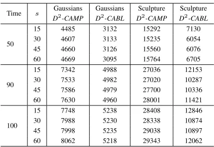
Table 1: Communication cost with varied values ofs

a worse clustering. For simplicity, we used the total number of edges communicated as the communication cost, which approximates the total number of bits by a logarithmic fac-tor. We implemented all five algorithms in Matlab programs, and conducted the experiments on a machine equipped with Intel i7 7700 2.8GHz CPU, 8G RAM and 1T disk storage.

The details of the datasets we used in the experiments are described as follows. TheGaussiansdataset consists of 800 nodes and 47,897 edges. Each point from each of four clus-ters is sampled from an isotropic Gaussians of variance 0.01. We consider each point to be a node in constructing the sim-ilarity graph. For every two nodesuandvsuch that one is among the 100-nearest points of the other, we add an edge of weightW(u, v) = exp{−||u−v||2

2/2σ2}withσ = 1. The numberkof clusters is 4. For theSculpturedataset, we used a22×30version of a photo of The Greek Slave3, and it contains 1980 nodes and 61,452 edges. We consider each pixel to be a node by mapping each pixel to a point inR5_{, i.e.}

(x, y, r, g, b), where the last three coordinates are the RGB

values. For every two nodesuandvsuch thatu(v) is among the 80-nearest points of v (u), we add an edge of weight

W(u, v) =exp{−||u−v||2

2/2σ2}withσ= 20. The num-berkof clusters is 3.

In the problem studied, the site and the time point each edge comes is arbitrary. Therefore, we make that the edges of nodes with smaller x coordinates have smaller arrival times than the edges of nodes with largerxcoordinates. In-tuitively, this results in that the edges of nodes on the left side come before the edges of nodes on the right side. This helps us to easily monitor the changing of the clustering re-sults. Independently, the site every edge comes is randomly picked from the interval[1, s].

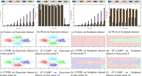
Experimental Results.As the baseline setting, we selected the total number of time pointst = 10and the total num-ber of sitess = 30. The communication cost and NCut of different algorithms on both datasets are shown in Fig. 2. On both datasets, the communication cost ofD2_-CAMP_and

D2-CABLare much smaller thanCNTRL,STMPandSTBL. Specifically, on Gaussians dataset, the communication cost ofD2-CAMPcan be only 4% of that ofSTMPand on

aver-3

(7)

1 2 3 4 5 6 7 8 9 10

Time point

0 0.5 1 1.5 2 2.5

Communication cost

105

D2-CAMP D2-CABL CNTRL STMP STBL

(a) Comm. on Gaussians dataset

1 2 3 4 5 6 7 8 9 10

Time point

0 0.5 1 1.5 2 2.5 3

Normalized cut

D2

-CAMP D2

-CABL CNTRL STMP STBL

(b) NCut on Gaussians dataset

1 2 3 4 5 6 7 8 9 10

Time point

0 0.5 1 1.5 2 2.5 3

Communication cost

105

D2-CAMP D2-CABL CNTRL STMP STBL

(c) Comm. on Sculpture dataset

1 2 3 4 5 6 7 8 9 10

Time point

0 0.5 1 1.5 2 2.5

Normalized cut

D2

-CAMP D2

-CABL CNTRL STMP STBL

(d) NCut on Sculpture dataset

-1 -0.5 0 0.5 1 1.5 2 2.5 3 -2

-1 0 1 2

(e)CNTRLon Gaussians dataset

at time point 9

-1 -0.5 0 0.5 1 1.5 2 2.5 3 -2

-1 0 1 2

(f) D2-CAMP on Gaussians

dataset at time point 9

0 5 10 15 20 25 30 0

5 10 15 20 25

(g)CNTRL on Sculpture dataset

at time point 9

0 5 10 15 20 25 30 0

5 10 15 20 25

(h) D2-CAMP on Sculpture

-1 -0.5 0 0.5 1 1.5 2 2.5 3 -2

-1 0 1 2

(i)CNTRLon Gaussians dataset

at time point 10

-1 -0.5 0 0.5 1 1.5 2 2.5 3 -2

-1 0 1 2

(j) D2-CAMP on Gaussians

0 5 10 15 20 25 30 0

5 10 15 20 25

(k)CNTRL on Sculpture dataset

at time point 10

0 5 10 15 20 25 30 0

5 10 15 20 25

(l) D2-CAMP on Sculpture

Figure 2: Communication cost, NCut and clustering results in the baseline setting

Time t Gaussians Gaussians Sculpture Sculpture

D2_-CAMP _D2_-CABL _D2_-CAMP _D2_-CABL

50%

10 4562 3127 15078 5998 30 4645 3126 15278 6063 100 4607 3133 15235 6054 300 4620 3113 15269 6064

90%

10 7467 4979 26699 10202 30 7581 4983 27012 10278 100 7533 4982 27020 10287 300 7618 4958 27042 10299

100%

10 7917 5225 28046 10779 30 8045 5234 28278 10847 100 7988 5230 28338 10874 300 8031 5211 28345 10869

Table 2: Communication cost with varied values oft

age 16% of that ofCNTRL. The communication cost ofD2 -CABLis on average 11% ofCNTRLand can be only 12% of that ofSTBL.STMPhas communication cost even much larger thanCNTRL.D2-CABLhas a smaller communication cost thanD2-CAMP. On Sculpture dataset, the communica-tion cost ofD2-CAMPcan be only 11% of that ofSTMPand is on average 49% of that ofCNTRL. The communication cost ofD2-CABLcan be only 15% of that ofSTBLand is on average 21% of that ofCNTRL. Similar toSTMP,STBLalso has communication cost larger thanCNTRL.D2-CABLhas a much smaller communication cost thanD2-CAMPand the difference here is larger than in Gaussians dataset.

For both datasets, all algorithms have comparable NCut at every time point, except that on Gaussians dataset, at

the time point 9,D2_-CABL_{has a slightly larger NCut. This} could be due to that D2-CABLis a randomized algorithm with high success probability. In Fig. 2(e-l), the clustering results of CNTRLandD2-CAMPon both datasets at time points 9 and 10 are visually very similar. (The same clus-ter colors in different figures do not have relation.) But for Sculpture dataset at the time point 9, the clustering result of

D2_-CAMP_{visually looks even more reasonable.}

We then varied the value ofsfrom 15 to 60 with a step of 15 or the value of t from 10 to 300 with a factor of 3 while keeping the other parameters unchanged as in the baseline setting. Due to limit of space, we only show the resultant communication cost of D2_-CAMP_and_D2_-CABL on both datasets in Tables 1 and 2. But the complete results are referred to Appendix. When we varied the value ofs, the communication cost ofD2-CAMPincreases roughly linearly with the increase of the value ofsfrom 15 to 60, while that ofD2_-CABL_{do not obviously increase with the value of}_s_. These observations are consistent with their theoretical com-munication costO˜(ns)andO˜(n+s), respectively. When we varied the value of t, both the communication cost of

D2_-CAMP_and_D2_-CABL_{roughly keep the same, also} sup-porting our theory above.

Finally, we tested the performance ofD2-CAMPandD2 -CABLfor dynamic graph streams. We randomly chose 5% of edges to delete at a random time point after their arrival. This increases the communicate cost ofCNTRLby 5% asCNTRL

sends every deletion to the coordinator/blackboard. How-ever, the communication cost ofD2-CAMPandD2-CABL

(8)

every time point have NCut comparable to that ofCNTRL. Due to limit of space, we refer to Fig. 1 in Appendix.

5 Conclusion and Future Work

In this paper, we study the problem of how to efficiently perform graph clustering over modern graph data that are often dynamic and collected at distributed sites. We de-sign communication-optimal algorithmsD2-CAMPandD2 -CABLfor two different communication models and prove their optimality rigorously. Finally, we conducted extensive simulations to confirm thatD2_-CAMP_and_D2_-CABL signif-icantly outperform baseline algorithms in practice. As the future work, we will study whether and how we can achieve similar results for geometric clustering, and how to achieve better computational bounds for the studied problems. We will also study other related problems in the distributed dynamic setting such as low-rank approximation (Bring-mann, Kolev, and Woodruff 2017), source-wise and stan-dard round-trip spanner constructions (Zhu and Lam 2017; 2018) and cut sparsifier constructions (Abraham et al. 2016).

Acknowledgments

This work was partially supported by NSF grants DBI-1356655, CCF-1514357, IIS-1718738, as well as NIH grants R01DA037349 and K02DA043063 to Jinbo Bi.

References

Abraham, I.; Durfee, D.; Koutis, I.; Krinninger, S.; and Peng, R. 2016. On fully dynamic graph sparsifiers. InProceedings of FOCS

Conference, 335–344.

Althofer, I.; Das, G.; Dobkin, D.; Joseph, D.; and Soares, J. 1993. On sparse spanners of weighted graphs. Discrete Computational

Geometry9:81–100.

Anagnostopoulos, A.; Lacki, J.; Lattanzi, S.; Leonardi, S.; and Mahdian, M. 2016. Community detection on evolving graphs.

InProceedings of NIPS Conference, 3530–3538.

Arbelaez, P.; Maire, M.; Fowlkes, C.; and Malik, J. 2011. Contour detection and hierarchical image segmentation.IEEE Transactions

on Pattern Analysis and Machine Intelligence33(5):898–916.

Baston, J.; Spielman, D.; and Srivastava, N. 2012. Twice-ramanujan sparsifiers. SIAM Journal on Computing41(6):1704– 1721.

Bringmann, K.; Kolev, P.; and Woodruff, D. 2017. Approximation algorithms forl0-low rank approximation. InProceedings of NIPS

Chen, J.; Sun, H.; Woodruff, D.; and Zhang, Q. 2016. Communication-optimal distributed clustering. InProceedings of

NIPS Conference, 3720–3728.

Cohen, M.; Musco, C.; and Pachocki, J. 2016. Online row sam-pling. In Proceedings of APPROX-RANDOM Conference, 7:1– 7:18.

Cormode, G.; Muthukrishnan, S.; and Wei, Z. 2007. Conquering the divide: continuous clustering of distributed data streams. In

Proceedings of ICDE Conference, 1036–1045.

Dijkstra, E. 1959. A note on two problems in connexion with graphs.Numerische Mathematik1(1):269–271.

Elkin, M. 2011. Streaming and fully dynamic centralized algo-rithms for constructing and maintaining sparse spanners. ACM

Transactions on Algorithms7(2):20.

Giatsidis, C.; Malliaros, F.; Thilikos, D.; and Vazirgiannis, M. 2014. CORECLUSTER: A degeneracy based graph clustering framework. InProceedings of AAAI Conference, 44–50.

Hui, P.; Yoneki, E.; Chan, S.; and Crowcroft, J. 2007. Distributed communicty detection in delay tolerant networks. InProceedings of 2nd ACM/IEEE International Workshop on Mobility in Evolving

Internet Architecture.

Jian, X.; Lian, X.; and Chen, L. 2018. On efficientl detecting overlapping communities over distributed dynamic graphs. In

Pro-ceedings of ICDE Conference.

Kapralov, M.; Lee, Y.; Musco, C.; Musco, C.; and Aaron, S. 2014. Single pass spectral sparsification in dynamic streams. In

Proceed-ings of FOCS Conference, 561–570.

Kelner, J., and Levin, A. 2013. Spectral sparsification in the semi-streaming setting.Theory of Computing Systems53(2):243–262. Kim, S.; Nowozin, S.; Kohli, P.; and Yoo, C. 2011. Higher-order correlation clustering for image segmentation. InProceedings of

NIPS Conference, 1530–1538.

Lee, Y., and Sun, H. 2017. An SDP-based algorithm for linear-sized spectral sparsification. InProceedings of STOC Conference, 678–687.

Lee, J.; Gharan, S.; and Trevisan, L. 2014. Multiway spectral partitioning and higher-order Cheeger inequalities. Journal of the ACM61(6):37.

Li, M.; Miller, G.; and Peng, R. 2013. Iterative row sampling. In

Proceedings of FOCS Conference, 127–136.

Maier, M.; Luxburg, U.; and Hein, M. 2009. Influence of graph construction on graph-based clustering measures. InProceedings

of NIPS Conference, 1025–1032.

Ng, A.; Jordan, M.; and Weiss, Y. 2001. On spectral clustering: analysis and an algorithm. In Proceedings of NIPS Conference, 849–856.

Peleg, D., and Schaffer, A. 1989. Graph spanners. Journal of

Graph Theory13(1):99–116.

Peng, R.; Sun, H.; and Zanetti, L. 2015. Partitioning well-clustered graphs: spectral clustering works! InProceedings of COLT

Con-ference, 1423–1455.

Phillips, J.; Verbin, E.; and Zhang, Q. 2016. Lower bounds for number-in-hand multiparty communication complexity, made easy.

SIAM Journal on Computing45(1):174–196.

Shi, J., and Malik, J. 2000. Normalized cuts and image segmenta-tion. IEEE Transactions on Pattern Analysis and Machine

Intelli-gence22(8):888–905.

Spielman, D., and Srivastava, N. 2011. Graph sparsification by effective resistances. SIAM Journal on Computing 40(6):1913– 1926.

Spielman, D., and Teng, S.-H. 2011. Spectral sparsification of graphs.SIAM Journal on Computing40(4):981–1025.

Sun, H., and Zanetti, L. 2017. Distributed graph clustering and sparsification.https://arxiv.org/abs/1711.01262.

Tian, F.; Gao, B.; Cui, Q.; Chen, E.; and Liu, T.-Y. 2014. Learning deep representations for graph clustering. InProceedings of AAAI

Worldwidewebsize. 2018. http://www.worldwidewebsize.com/. [Online; accessed 05-07-2018].

Yang, W., and Xu, H. 2015. A divide and conquer framework for distributed graph clustering. InProceedings of ICML Conference, 504–513.

Zhu, C., and Lam, K.-Y. 2017. Source-wise round-trip spanners.

Information Processing Letters124(C):42–45.