The Thirty-Third AAAI Conference on Artificial Intelligence (AAAI-19)
Interpreting Deep Models for Text Analysis
via Optimization and Regularization Methods
Hao Yuan
Washington State University [email protected]
Yongjun Chen
Washington State University [email protected]
Xia Hu
Texas A&M University [email protected]
Shuiwang Ji
Texas A&M University [email protected]
Abstract
Interpreting deep neural networks is of great importance to understand and verify deep models for natural language pro-cessing (NLP) tasks. However, most existing approaches only focus on improving the performance of models but ignore their interpretability. In this work, we propose an approach to investigate the meaning of hidden neurons of the con-volutional neural network (CNN) models. We first employ saliency map and optimization techniques to approximate the detected information of hidden neurons from input sentences. Then we develop regularization terms and explore words in vocabulary to interpret such detected information. Experi-mental results demonstrate that our approach can identify meaningful and reasonable interpretations for hidden spatial locations. Additionally, we show that our approach can de-scribe the decision procedure of deep NLP models.
Introduction
Deep neural networks have shown great success in many NLP tasks, such as sentence classification (Kim 2014; Zhang, Zhao, and LeCun 2015), natural language gener-ation (Yu et al. 2017; Lin et al. 2017), machine transla-tion (Vaswani et al. 2017; Gehring et al. 2016) and visual question answering (Wang and Ji 2018). Most existing ap-proaches treat deep neural networks as black-boxes and only focus on the performance. Without understanding the work-ing mechanisms of neural networks, deep models cannot be fully trusted, since we do not know how and why decisions are made. However, due to the complex structures of deep neural networks, it is challenging to interpret deep models and their behaviors, especially for NLP tasks that deal with discrete data.
Most existing approaches for interpreting NLP models only investigate the relationships between input sentences and output decisions to explore which input words are more important to make decisions (Lei, Barzilay, and Jaakkola 2016; Li et al. 2015). However, the inner workings of net-works should also be studied to answer important questions regarding hidden layers, such as which hidden units are more important for a decision and why they are important. To the
Copyright c2019, Association for the Advancement of Artificial Intelligence (www.aaai.org). All rights reserved.
best of our knowledge, there are no related studies focusing on the interpretation of hidden neurons of NLP models.
In this paper, we propose an approach to interpret and un-derstand deep NLP models. Specifically, we focus on convo-lutional neural networks (CNN) (Krizhevsky, Sutskever, and Hinton 2012) for sentence classification tasks. Our approach employs gradient-based approaches (Simonyan, Vedaldi, and Zisserman 2013) and optimization techniques (Erhan et al. 2009) to select spatial locations with high contribution to the decision from hidden layers and study what is detected by these locations. We propose to approximately interpret the meaning of detected information using the nearest neigh-bors of the optimized representation based on the special property of word representations, which imply that words with semantically similar meanings are embedded to nearby points (Mikolov et al. 2013). Experimental results demon-strate that our approach can obtain reasonable and mean-ingful interpretation for hidden units. It is shown that our approach can explain the decision process in NLP models.
Background and Related Work
Most of the existing interpretation approaches are proposed to investigate deep models in computer vision rather than the NLP area. The saliency map techniques study which input pixels are more important to the final decision (Simonyan, Vedaldi, and Zisserman 2013; Du, Liu, and Hu 2018; Du et al. 2018). The importance of different pixels can be approx-imated by the gradient of output score with respect to the inputs (Zeiler and Fergus 2014; Springenberg et al. 2014; Mordvintsev, Olah, and Tyka 2015). The similar idea was applied to NLP models to study which input words con-tribute more to the prediction (Li et al. 2015). However, such techniques only provide word-level interpretation while dif-ferent words are highly correlated to convey a meaning.
lay-ers, such as maximizing the activation values of neurons or maximizing the score of a class. The optimized input can then be visualized as abstracted images to reflect the mean-ing. However, such a technique cannot be directly applied to NLP models since word representations are discrete and the meaning cannot be abstracted. Thus the optimized input is difficult to interpret. By combining the above two tech-niques, (Olah et al. 2018) investigate the meaning of hid-den layers to interpret models for image classification tasks. However, as we mentioned above, the optimized input is a sequence of abstract vector representations and cannot be visualized as abstracted texts. We propose an approach to approximately interpret the high-level meaning of the opti-mized input by selecting the neighbors of these vector rep-resentations from the embedding space.
Methods
As discussed above, it is not enough to only build saliency maps on input sentences to visualize word-level interpreta-tion, since different words may combine together to convey a meaning. In addition, without investigating the hidden lay-ers, we still do not understand how the hidden neurons work, and neural networks remain a black box. To better under-stand deep NLP models, we propose an approach to focus on the contribution and meaning of hidden neurons, thereby allowing us to visually interpret the decision process.
Visual Interpretation of Hidden Units
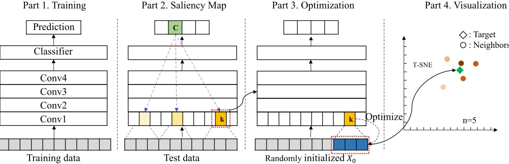
In this work, we investigate the interpretation of CNN mod-els for sentence classification tasks in NLP. The general structure of CNN models we study is shown in Figure 1. Given an input sentence, it first passes through an embed-ding layer and several convolutional layers. Then it is fed into a max-pooling layer and a fully-connected layer with softmax function to make predictions.
Intuitively, we wish to investigate the hidden units of a deep NLP model so that we can answer three questions; those are, which hidden spatial locations are more important to decisions? what is detected by these spatial locations from input sentences? and what is the meaning of the detected in-formation? However, there are two main challenges for an-swering these questions; those are, how to explore what is detected by hidden units? and how to interpret the detected information? Existing approaches in computer vision cannot be directly applied since word representations are discrete from each other and cannot be abstracted as images.
We first combine the idea of saliency map and optimiza-tion to answer the quesoptimiza-tion of what is detected by hidden units. Based on the property of word representations, we propose to approximately interpret the meaning of detected information using the nearest neighbors of the optimized representation. Then we develop regularization terms to help interpretation. Generally speaking, the interpretation proce-dure consists of three main steps. First, we employ gradient-based approaches to estimate the contributions of different spatial locations in a hidden layer. Based on the magnitude of contributions, the spatial locations are sorted, and those with high contribution are selected to be interpreted in the
following steps. Second, to obtain what is detected by differ-ent spatial locations in hidden layers, we iteratively update a randomly initialized input via optimization. Finally, the op-timized input is a sequence of numerical vectors but such abstract values are hard to interpret. Based on the property of word representations that words with semantically similar meanings are embedded to nearby points, we design regular-ization terms to encourage different vectors in the optimized input to be similar to each other. Then we explore the near-est neighbors (Altman 1992) in term of cosine similarity to approximately represent the meaning of the target spatial lo-cation. The general logic flow of our approach is illustrated in Figure 1.
Saliency Maps for Hidden Units
Since there are a large number of neurons in hidden layers, it is not possible to interpret each neuron. Hence we em-ploy saliency map techniques to select spatial locations with high contributions for further interpretation. The saliency map acts like a heatmap, where saliency scores are esti-mated by the first order derivatives and reflects the contribu-tion of different neurons. While most of existing approaches build saliency maps to explore the contribution of individual words in input sentences, we study the importance of differ-ent hidden spatial locations instead.
Formally, for an input sentenceX, the model predicts that
it belongs to classcand produces a class scoreSc. Letaij
represents the activation vector of the spatial location i of
layerj, and its dimension is equal to the number of
chan-nels. Also letAjdenotes the activations of layerj, which is a
matrix, where each column corresponds to one spatial
loca-tion. The relationship between the scoreScandAjis highly
non-linear due to the non-linear functions in deep neural net-works. Inspired by the strategy in recent work (Li et al. 2015; Simonyan, Vedaldi, and Zisserman 2013), we compute the first-order Taylor expansion as a linear function to approxi-mate the relationship as
Sc≈Tr(w(Aj)TAj) +b, (1)
whereTr(·)denotes the trace of a matrix andw(Aj)is the
gradient of class scoreSc with respect to the layerj. Such
gradient can be obtained by using the first order derivative
ofScwith respect to the layerAjas
w(Aj) =
∂Sc
∂Aj
. (2)
For the spatial location iin the layer j, the gradient of
Sc with respect to this spatial location is theithcolumn of
w(Aj), denoted asw(Aj)i. Then the saliency score of this
location Scorec(X)i,jis calculated using linear
approxima-tion:
Scorec(X)i,j =w(Aj)i·aij, (3)
where·refers to the dot product of vectors.
Part 1. Training Part 2. Saliency Map Part 3. Optimization Part 4. Visualization
C
Conv4 Conv3 Conv2 Classifier
Optimize
Training data Test data Randomlyinitialized𝑋"
: Target
n=5 T-SNE
Conv1 Prediction
: Neighbors
k k
Figure 1: Illustration of the overall pipeline of our approach. Part1shows the general structure of the CNN model that we try
to investigate. After training, we first build saliency maps for different hidden spatial locations, where saliency scores reflect
contributions to the final decision. As the example shown in Part2, the CNN model classifies the test sentence to classc(shown
in green). For the conv1 layer, the saliency score is computed for each spatial location, and three spatial locations are selected (highlighted in yellow). Next, for each selected location, optimization technique is employed to determine what is detected
from the test sentence. As shown in Part3, for the spatial locationk, a randomly initialized inputX0is fed to the network and
we iteratively updateX0towards the objective function shown in Equation 6. Finally, based on the receptive field of location
k(shown in blue with red bounding box), we obtain an overall representation for this receptive field. We search the vocabulary
and select word representations with high similarity to the overall representation. Then, the t-SNE is employed to visualize
these representations, as shown in Part4.
how much one spatial location contributes to the final class score. In addition, after training, the weights and parameters
in the model are fixed so that the gradient ofScwith respect
to a specific spatial location is fixed and does not depend on the input. By using the linear approximation, the saliency score becomes input-dependent.
Input Generation via Optimization
By employing the saliency map technique, we can select spatial locations with high influence on the final decision. However, it is still not clear why they are important. In or-der to explore this direction, we propose to use optimiza-tion techniques to understand what is detected from the in-put sentence by these spatial locations. The key idea of op-timization techniques for interpretation is to iteratively up-date a randomly initialized input towards an objective func-tion. Such optimization procedure is similar to the training of deep neural networks. The main difference is that in such optimization techniques, the parameters of the networks are fixed but the input is optimized. When maximizing the acti-vation value of a certain neuron, the optimized input reflects the pattern that this neuron tries to detect (Zeiler and Fergus 2014; Erhan et al. 2009). The activation value of each neu-ron shows the strength of the pattern detected from inputs.
For the neuronkin the spatial locationiof hidden layerj,
we can obtain an optimized input Xijk and the activation
valueaijk. When considering spatial locations as a whole,
what is detected can be approximated using a weighted sum
ofXijkandaijkas
Xij = n
X
k=1
aijkXijk, (4)
wherenis the number of neurons in the spatial locationiof
layerj, which is equal to the number of channels.
Such approximations are not efficient since the number of channels can be large, and we need to obtain an opti-mized input for each neuron. Furthermore, it is challenging to add regularization since the optimized input is generated for each neuron separately. Hence, we propose to incorpo-rate the activation vector of a spatial location and optimize the input for the whole spatial location. Formally, for a spa-tial locationiof layerj, letaij represents its activation
vec-tor given the input sentenceX. We randomly initialize
an-other inputX0and feed it to the network. For the same
spa-tial location, we obtain another activation vectora0ij. Then
we iteratively update the inputX0towards the following
ob-jective function:
maxaij·a0ij, (5)
where·refers to the dot product of vectors.
Regularization
In Equation 5, there is no regularization term for optimiza-tion. However, without any regularization, the updating
pro-cedure will not converge since the inputX0can be updated
without any constraint, and the targetaij·a0ijkeeps
increas-ing. Hence, we addL2regularization to the objective
func-tion. In addition, in order to interpret the optimized input, we propose to add another regularization term, known as the similarity regularization, to make the optimized inputs read-ily interpretable.
Formally, let Xc0 denotes the receptive field of the
spa-tial location we try to investigate, and l andrare the
haveX0c = [x0l,· · · , x0i,· · ·, x0r], wherex0i denotes the
ith column ofX0. By adding the regularization terms, the
objective function becomes
maxaij·a0ij−λ1
X0c
2
2+λ2Sim(X0c), (6)
where· denotes the dot product of vectors, Sim(·) is the
similarity term, andλ1, λ2are regularization parameters.
L2Term: By adding theL2regularization, the
optimiza-tion procedure converges much faster. Furthermore, theL2
term encourages features with high contributions to the tar-getaij·a0ijto increase more than others. This is beneficial,
since features of high importance can better represent the meaning of hidden spatial locations.
Similarity Term: Intuitively, we try to assign each spatial location an estimated meaning to represent what is detected from the input sentence. After optimization, we obtain mul-tiple vector representations. However, such representations may be very different from each other. In this case, it is chal-lenging to find an overall representation for them. Based on the property of word representation that words with seman-tically similar meanings localize closer in the embedding space (Mikolov et al. 2013; Li et al. 2015), we propose the similarity regularization for optimization, which encourages
different vector representations in optimizedX0to be
sim-ilar to each other. In this way, these vector representations are encouraged to have similar semantically meanings when mapping back to the word space. Formally, the similarity term is defined as
Sim(X0c) = 1
N
X
∀i,j
x0i
kx0ik2
· x0j kx0jk2
, (7)
where·refers to dot product of vectors,N =r−l+ 1and
i, j∈[l, r].
Visualization of Optimized Inputs
By combining saliency maps and optimization, we know which spatial locations in hidden layers contribute most to the final decision. We also obtain an optimized input for each selected hidden spatial location to represent what is de-tected by this location. However, the optimized input con-sists of several numerical vectors and is still hard to inter-pret. It is challenging because words representations are dis-crete so that the optimized representations cannot be mapped to words directly. We propose to find representative words whose vector representations have high cosine similarity with the optimized input as an estimation of the meaning.
Given an optimized inputX0, based on the spatial
loca-tion we can obtain its receptive field with respect toX0,
de-noted as X0c = [x0l,· · · , x0i,· · ·, x0r]. Since we employ
the similarity regularization term, different representations
x0iare encouraged to be similar. Additionally, in the case of
word embedding, similar representations lead to similar se-mantic meanings. Hence, it is reasonable to take an average of these representations as an overall approximation as
xoverall=
1
N
r
X
i=l
x0i. (8)
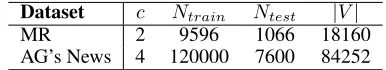
Dataset c Ntrain Ntest |V|
MR 2 9596 1066 18160
AG’s News 4 120000 7600 84252
Table 1: The summary statistics of the MR dataset and the
AG’s News dataset. In the table,crepresents the number of
classes,Ntraindenotes the number of training examples in
the dataset,Ntest is the number of test examples, and |V|
denotes the size of vocabulary.
It is impossible to find the exact meaning for xoverall.
Instead, we study the neighbors of xoverall in the
embed-ding space. We believe the neighbors share similar
high-level semantic meaning withxoverall. Specifically, we
com-parexoverallwith different word representations in the
vo-cabulary using cosine similarity and obtain the top words and their corresponding representations. By studying the se-mantic meaning of these neighbors, we can understand the high-level meaning of the detected information by this spa-tial location. Finally, these representations can be visualized in the 2D space via dimension reduction techniques, such as t-SNE (Maaten and Hinton 2008) and principal component analysis (Wold, Esbensen, and Geladi 1987).
Experimental Studies
To demonstrate the effectiveness of our approach, we eval-uate our methods both quantitatively and qualitatively. We first introduce two datasets we are using and the setup of the experiments in detail. Next, we report the interpretation re-sults for several sentence examples. Finally, we present the quantitative evaluations of our methods.
Datasets
We conduct experiments to show the effectiveness of our ap-proach based on two NLP datasets; namely the MR dataset and AG’s News dataset. We report the summary statistics of these two datasets in Table 1.
MR Dataset: The MR dataset1 contains movie review data for sentiment analysis. Each sample in the dataset is a one-sentence movie review and labeled with “positive” or “negative”.
AG’s News Dataset: The AG’s News dataset2 is structed from AG’s corpus of news articles. The dataset con-tains the largest 4 classes of news in the original AG’s cor-pus, where only the title and description are used (Zhang, Zhao, and LeCun 2015). The label of each news example depends on the topic of the news, which can be “World”, “Sports”, “Business” or “Sci/Tech”. Each class has 30,000 training examples and 1,900 testing examples.
Experimental Setup
In this section, we introduce the CNN model that we inves-tigate in this work. We then discuss the interpretation setup
1
https://www.cs.cornell.edu/people/pabo/movie-review-data/
2
http://www.di.unipi.it/∼gulli/AG corpus of news articles.
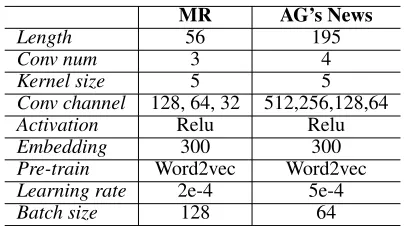
MR AG’s News
Length 56 195
Conv num 3 4
Kernel size 5 5
Conv channel 128, 64, 32 512,256,128,64
Activation Relu Relu
Embedding 300 300
Pre-train Word2vec Word2vec
Learning rate 2e-4 5e-4
Batch size 128 64
Table 2: The CNN models we used for the MR dataset and AG’s News dataset. Different columns refer to the network
settings for different dataset. Length: the length of input
sentence;Conv num: the number of 1D convolutional
lay-ers in the model;Conv channel: the number of channels for
convolutional layers;Activation: activation function in
con-volutional layers; Embedding: dimension of word
embed-ding;Pre-train: the type of pre-trained word embedding
em-ployed.
in detail. Finally, we discuss the preprocessing procedure for text inputs.
CNN Model: We build CNN models for both datasets, and the overall structures are shown in Part 1 of Figure 1. The input sentence is padded to the same length and fed into the embedding layer, where the word2vec word embedding is employed (Mikolov et al. 2013). Then several 1D convo-lutional layers (LeCun et al. 1998) and a max-pooling layer are applied. Finally, a fully-connected layer with the softmax function produces the predictive decision. Detailed descrip-tions of models are given in Table 2.
Interpretation: After training, the parameters and vocab-ulary in CNN models are saved for interpretation. These trained parameters in CNN models are reused and fixed during the interpretation procedure. Given a test sentence,
the saliency map technique returns the top mspatial
loca-tions for a hidden layer. We setmequal to 3 in our
experi-ments and focus on the first hidden layer. The input in opti-mization is randomly initialized using the Xavier initializa-tion method (Glorot and Bengio 2010). For the MR dataset,
the regularization parameters are set as λ1 = 0.004 and
λ2 = 0.02. For the AG’s News dataset, we setλ1 = 0.002
andλ2 = 0.01. We implement our approach using
Tensor-Flow and conduct our experiments on one Tesla K80 GPU.
The learning rate in optimization procedure is set to2×e−4
and we apply the Adam optimizer (Kingma and Ba 2014)
with momentum parametersβ1= 0.9andβ2= 0.999.
Preprocessing: The way to preprocess the text data is similar to the existing NLP application (Kim 2014). It is noteworthy that we do not convert words to lower case since the meaning of a word is case-sensitive.
Visual Interpretation Results
We first report the prediction accuracy of the CNN mod-els that we try to interpret. The results are shown in Ta-ble 3. The CNN models we build can achieve competi-tive or even better performance compared with the baseline
Dataset MR AG’s News
Our CNN model 79.96% 92.05%
Baseline CNN model 81.50% 91.45%
Table 3: Comparison of prediction accuracy between the CNN models we build and the baseline CNNs.
CNNs (Kim 2014; Zhang, Zhao, and LeCun 2015). The rea-son why we conduct such comparirea-son is that we wish to show the CNNs we investigate are models with reasonable performance. Next, we present the visual interpretation re-sults to demonstrate the effectiveness of our approach.
MR Dataset: For the MR dataset, we show the
visualiza-tion results for two testing examples; those are,“As a good
old fashioned adventure for kids spirit stallion of the cimar-ron is a winner”; and“Plays like one of those conversations that comic book guy on the simpsons has”. Clearly, the first example is a positive review while the second one is a neg-ative one. Both of them are correctly classified by the CNN models.
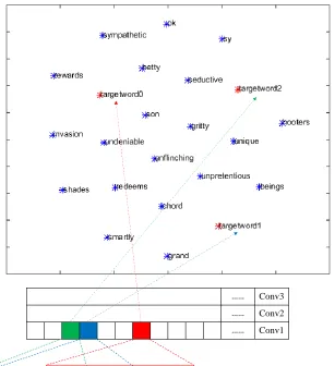
The visual interpretation result of the first example is shown in Figure 2. As demonstrated, three spatial locations (grids in red, blue and green) of the first convolutional layer are selected based on their saliency scores. The bounding boxes reflect the receptive fields of these spatial locations with respect to the input. The receptive fields contain words like “good”, “fashioned”, “adventure”, and “spirit”, which are commonly used in positive movie reviews. In addition, the top part of Figure 2 shows the visual interpretation for se-lected hidden spatial locations. Most of the neighbors iden-tified by our approaches are positive adjectives, such as “unflinching”, “ok”, “smartly”, and “gritty”. We use these neighbors to represent the meanings of hidden spatial loca-tions so that the localoca-tions should be interpreted as positive meaning. This is consistent with their receptive fields and the final positive prediction. Such interpretation helps us un-derstand how the decision is made; that is, the information detected by these spatial locations is positive and these spa-tial locations have high contribution to the final decision so that the final prediction is positive.
In addition, we show the visualization result of the sec-ond MR example in Figure 3. Clearly, many words with negative meanings are selected to interpret the meaning of hidden spatial locations, such as “terribly”, “awkward”, “de-void”, “unwatchable” and “brainless”. Hence, these spatial locations can be interpreted as negative meaning, and it is consistent with the prediction. We also observe that most of neighbors are adjectives or adverbs.
AG’s News Dataset: Similarly, we show the interpreta-tion results for two examples from the AG’s News dataset. Both of them are correctly classified by CNN models.
The first example with label “sports” is “Looking at his
As a good old fashioned adventure for kids spirit stallion of the cimarron is a winner
…… Conv3
…… Conv2
…… Conv1
Figure 2: The visualization interpretation result for the first example for the MR dataset. The middle part of the figure shows the contribution of different spatial locations in hidden layers, where red color means highest contribution to the final decision; blue color refers to the second highest contribution; and green means the third highest contribution. The bounding boxes in different colors correspond to the receptive field of different spatial location. The top part shows the t-SNE visualization of the interpretation obtained by our approach. The interpretations of target spatial locations are marked as “targetword” and connected to the corresponding spatial locations by dash lines.
are names of famous players; “Toulouse ” and “Newcastle” are names of famous sports teams. One may argue that such names can be used in many areas and are not limited in topic “sports”. We claim that our interpretation results are based on the model and datasets where there are only four classes: “World”, “Sports”, “Business” and “Sci/Tech”. When only considering these four types of news, these names are highly related to “sports”. Hence, we believe the selected words are reasonable and consistent with the prediction.
The second example is“Jet Propulsion Lab – Scientists
have discovered irregular lumps beneath the icy surface of Jupiter’s largest moon, Ganymede”. Obviously, it belongs to topic “Sci/Tech”. The interpretation result is shown in Fig-ure 5. Similarly, the word selected by our approaches are highly related to “Sci/Tech” topic, such as “Solar”, “pro-torosaur”, “datacenter” and “Scientistcom”.
In addition, it is interesting that for the MR dataset, the in-terpretation results are mostly adjectives and adverbs while
the results of AG’s News data contains more nouns. This is reasonable since in movie review, the positive or nega-tive meaning is mostly expressed by adjecnega-tives and adverbs while the topic of a news is highly related to nouns. Such ob-servation also demonstrates that our approach provides rea-sonable interpretation based on the model and dataset. In conclusion, the words selected by our approach to interpret the hidden locations are meaningful and reasonable. They interpret the information detected from the input sentence. In addition, such interpretations help explain how the deci-sion is made and why the decideci-sion is made.
Evaluation of Interpretability
targetword0
comparison jonah
ricochets
irrelevant chosen
brainless
chen
sadly
unwatchable
targetword1
flounders
ship shifting
voices
targetword2
wishing painted
shakes
miserable
terribly awkward
anyway
devoid distressingly
Figure 3: The visualization interpretation result for the sec-ond example for the MR dataset. Only the final result is pre-sented due to space constraints.
Dataset MR AG’s News
Matching rate 0.934 0.843
Table 4: The matching rates for the MR dataset and AG’s News dataset.
introduce how we quantitatively evaluate the interpretation.
Given an input sentenceX, the model classifies it to classc.
We obtain the interpretation ofklocations with the highest
contribution to the decision. For each location we use them
nearest neighbors to represent its meaning. In this way, for
each input, we have a sentence withkmwords to interpret
the hidden layer, denoted asX0. If we feedX0to the same
network, we obtain another classification result c0. Ifc is
equal toc0, we call it a matching, and it means the
interpre-tation of hidden locations shares similar high-level meaning with the input. Here, we focus on the first hidden layer and
setk= 3andm= 5, .
We conduct such evaluation for the two datasets and the results are reported in Table 4. It is obvious that for both datasets, our method provides reasonable interpretation for most examples. In addition, our approach has better perfor-mance on the MR dataset. We believe the reason is that the length of input examples in the AG’s News is much greater than that of MR data. Then it is more challenging to use the interpretation of three locations to represent the meaning of whole input sentences.
Conclusion
Investigating hidden units in neural networks are of great im-portance to understand their working mechanisms. However, most current approaches focus on models for images tasks. It is challenging to understand the meaning of hidden units in NLP models, since word representations are discrete and
targetword0
Uthman Elarton
Sobering GLOOM
LEVEL
Toulouse
sharedcontent
Fahrenhorst
Olympics
Evidently
targetword1 Toni
whiner
Daye hushed verstatile
Felling targetword2
Newcastle
harbours extant
Sizemore
TOURNAMENT TITLE
excelled Youngstown
Figure 4: The visualization interpretation result of the first example for the AG’s News dataset.
targetword0
Delf
responsibly
Bofra SETS
Illegally
protorosaur
Scientistcom
SPAZIO Autonomous
Takeoff
targetword1
tinkerers Portend
datacentre
Scripting Battens
targetword2
Solar coinciding
Arrogance
Universe
DBs Hayashi
Panacea
infrared
Figure 5: The visualization interpretation result of the sec-ond example for the AG’s News dataset.
cannot be abstracted. In this work, we propose an approach to interpret deep NLP models. We first combine the saliency map and optimization techniques to explore the information detected by the most important hidden units in NLP mod-els. Then we propose to approximately interpret the mean-ing of detected information usmean-ing the nearest neighbors of the optimized representation based on the special property of word representations. Experimental results show that our approaches can identify reasonable interpretation for hidden locations, which shares similar high-level meaning with the input sentence. It is also shown that our method helps ex-plain how the decision and why the decision is made.
Acknowledgement
Founda-tion grant [IIS-1615035] and Defense Advanced Research Projects Agency grant [N66001-17-2-4031].
References
Altman, N. S. 1992. An introduction to kernel and
nearest-neighbor nonparametric regression. The American
Statisti-cian46(3):175–185.
Du, M.; Liu, N.; Song, Q.; and Hu, X. 2018. Towards ex-planation of dnn-based prediction with guided feature
inver-sion.arXiv preprint arXiv:1804.00506.
Du, M.; Liu, N.; and Hu, X. 2018. Techniques
for interpretable machine learning. arXiv preprint
arXiv:1808.00033.
Erhan, D.; Bengio, Y.; Courville, A.; and Vincent, P. 2009.
Visualizing higher-layer features of a deep network.
Univer-sity of Montreal1341(3):1.
Gehring, J.; Auli, M.; Grangier, D.; and Dauphin, Y. N. 2016. A convolutional encoder model for neural machine
translation.arXiv preprint arXiv:1611.02344.
Glorot, X., and Bengio, Y. 2010. Understanding the
diffi-culty of training deep feedforward neural networks. In
Pro-ceedings of the thirteenth international conference on artifi-cial intelligence and statistics, 249–256.
Kim, Y. 2014. Convolutional neural networks for sentence
classification.arXiv preprint arXiv:1408.5882.
Kingma, D. P., and Ba, J. 2014. Adam: A method for
stochastic optimization.arXiv preprint arXiv:1412.6980.
Krizhevsky, A.; Sutskever, I.; and Hinton, G. E. 2012.
Imagenet classification with deep convolutional neural
net-works. InAdvances in neural information processing
sys-tems, 1097–1105.
LeCun, Y.; Bottou, L.; Bengio, Y.; and Haffner, P. 1998. Gradient-based learning applied to document recognition. Proceedings of the IEEE86(11):2278–2324.
Lei, T.; Barzilay, R.; and Jaakkola, T. 2016. Rationalizing
neural predictions. arXiv preprint arXiv:1606.04155.
Li, J.; Chen, X.; Hovy, E.; and Jurafsky, D. 2015.
Visualiz-ing and understandVisualiz-ing neural models in nlp. arXiv preprint
arXiv:1506.01066.
Lin, K.; Li, D.; He, X.; Zhang, Z.; and Sun, M.-T. 2017.
Adversarial ranking for language generation. InAdvances
in Neural Information Processing Systems, 3155–3165. Maaten, L. v. d., and Hinton, G. 2008. Visualizing data using
t-sne. Journal of machine learning research9(Nov):2579–
2605.
Mahendran, A., and Vedaldi, A. 2015. Understanding deep
image representations by inverting them. arXiv preprint
arXiv:1412.0035.
Mikolov, T.; Chen, K.; Corrado, G.; and Dean, J. 2013. Ef-ficient estimation of word representations in vector space. arXiv preprint arXiv:1301.3781.
Mordvintsev, A.; Olah, C.; and Tyka, M. 2015.
Inception-ism: Going deeper into neural networks. Google Research
Blog. Retrieved June20(14):5.
Nguyen, A.; Yosinski, J.; Bengio, Y.; Dosovitskiy, A.; and Clune, J. 2016. Plug & play generative networks:
Condi-tional iterative generation of images in latent space. arXiv
preprint arXiv:1612.00005.
Nguyen, A.; Yosinski, J.; and Clune, J. 2015. Deep neural networks are easily fooled: High confidence predictions for
unrecognizable images. InProceedings of the IEEE
Confer-ence on Computer Vision and Pattern Recognition, 427–436. Olah, C.; Satyanarayan, A.; Johnson, I.; Carter, S.; Schubert, L.; Ye, K.; and Mordvintsev, A. 2018. The building blocks
of interpretability. Distill.
https://distill.pub/2018/building-blocks.
Olah, C.; Mordvintsev, A.; and Schubert, L. 2017.
Fea-ture visualization. Distill.
https://distill.pub/2017/feature-visualization.
Simonyan, K.; Vedaldi, A.; and Zisserman, A. 2013.
Deep inside convolutional networks: Visualising image
classification models and saliency maps. arXiv preprint
arXiv:1312.6034.
Springenberg, J. T.; Dosovitskiy, A.; Brox, T.; and Ried-miller, M. 2014. Striving for simplicity: The all
convolu-tional net.arXiv preprint arXiv:1412.6806.
Vaswani, A.; Shazeer, N.; Parmar, N.; Uszkoreit, J.; Jones, L.; Gomez, A. N.; Kaiser, Ł.; and Polosukhin, I. 2017.
At-tention is all you need. InAdvances in Neural Information
Processing Systems, 6000–6010.
Wang, Z., and Ji, S. 2018. Learning convolutional text
rep-resentations for visual question answering. InProceedings
of the 2018 SIAM International Conference on Data Mining, 594–602. SIAM.
Wold, S.; Esbensen, K.; and Geladi, P. 1987. Principal
com-ponent analysis. Chemometrics and intelligent laboratory
systems2(1-3):37–52.
Yu, L.; Zhang, W.; Wang, J.; and Yu, Y. 2017. Seqgan: Sequence generative adversarial nets with policy gradient.
InAAAI, 2852–2858.
Zeiler, M. D., and Fergus, R. 2014. Visualizing and
under-standing convolutional networks. InEuropean conference
on computer vision, 818–833. Springer.
Zhang, X.; Zhao, J.; and LeCun, Y. 2015. Character-level
convolutional networks for text classification. InAdvances