Singular Value Decomposition & Few Application

(1)

Singular Value Decomposition & Few

Application

1

Jajimogga Raghavendar,

2

V.Dharmaiah

1

Research Scholar,Department of Mathematics,Rayalaseema University Kurnool, Andhra Pradesh,India

2_{Department of Mathematics, Retd. Professor, Osmania University, Hyderabad, Telangana-500007}

Abstract—Singular Value Decomposition (SVD) is a tool for teaching linear algebra geomatrically. In Linear algebra SVD is very usefulin many cases in problem solving. Some of the applications of SVD are,Image processing, Population related problems, Least square approximation in Numerical methods, Dimension reduction, Low rank data’s storage, Education related problems, Data composition. This paper discuss about fewer applications.

Keywords—SVD, Least Square Approximation, Education & Population Related Problems.

1. Introduction

This section introduces the hanger stretcher and aligner matrices. Any matrix can be written as the product of hanger, stricter and an aligner matrix. A 2D perpendicular frame consists of perpendicular circular unit vector which can be specified by an angle𝛼. As an example consider the unit vectors

𝑉1= (𝑐𝑜𝑠𝛼, 𝑠𝑖𝑛𝛼)

𝑉2= [cos

𝜋

2+ 𝛼 , sin 𝜋

2+ 𝛼 ]

𝑉1 .. 𝑉2= 0

Using these two perpendicular vectors as column or rows we can define respective hanger or the aligner matrix

1.1 Hanger Matrices

The hanger matrix determined by 𝐻 =

𝑐𝑜𝑠𝛼 cos 𝜋₂+ 𝛼

𝑠𝑖𝑛𝛼 sin 𝜋₂+ 𝛼

Set the angle𝛼 for the matrix H to 𝛼 =𝜋

2

Consider the ellipse

𝑥 𝜃 = 2 𝑐𝑜𝑠𝜃

𝑦 𝜃 = 1.5 𝑠𝑖𝑛𝜃In parametric form

Fig 1 Perpendicular vector 𝛼 =𝜋₄together with an ellipse..

The point on the ellipse are defined by the unit vector 1,0 and 0,1

𝑥 𝜃 , 𝑦 𝜃 = 𝑥 𝜃 1,0 + 𝑦 𝜃 [0,1]

∴ This means that 𝑥(𝜃) units in the direction of (1, 0) and 𝑦 𝜃 units in the direction of (0,1). Hung ellipse 𝜃 = 𝑥 𝜃 𝑉1+ 𝑦 𝜃 𝑉2

(2)

𝑐𝑜𝑠𝛼 cos 𝜋

2+ 𝛼

𝑠𝑖𝑛𝛼 sin 𝜋

2+ 𝛼

_cos𝑐𝑜𝑠𝛼𝜋 𝑠𝑖𝑛𝛼

2+ 𝛼 sin

𝜋

2+ 𝛼 =

1 0 0 1

1.2 Diagonal matrices X-Y-streching

Consider the diagonalmatrix 𝐷 = 3 0

0 2 which multiplying every point of the unit circle given of parametric

form, the result is shown in fig 2.

Where it can be seen that all measurements along the X–axis have been stretching by a factor of 3(the X stretch

factor) and all measuring matrix along the Y-axis by a factor of 2 the Y stretch factor)

To invert stretcher matrix D

𝐷−1₌

1

3 0

0 1

2

2. SVD Application

The SVD analyses enhance the teaching of linear algebra concepts and it is explain the definition of the matrix on a curve when the inverse of a matrix does not exists.

2.1 Theorem: The image of the unit circle in ℝ2 by an invertible 2 × 2 matrix is an ellipse with center at the origin.

Proof Denote the invertible matrix by 𝑀 = 𝑎 𝑏

𝑐 𝑑 , 𝑎𝑑 − 𝑏𝑐 ≠ 0 (2.1.1)

Then 𝑀−1 = 1

𝑎𝑑 −𝑏𝑐 𝑑

−𝑏

−𝑐 𝑎

𝑀Maps the unit circle to 𝑢_{𝑣 = 𝑀}𝑥_{𝑦 : 𝑥}2+ 𝑦2= 1

The equation of this set 𝑢, 𝑣 space is 𝑀−1 𝑢_𝑣

2

= 1

Plugging in the form for 𝑀−1 yields the equation

1

𝑎𝑑 − 𝑏𝑐 2 𝑑𝑢 − 𝑏𝑣, −𝑐𝑢 + 𝑎𝑣 2= 1

Expanding yields

1

𝑎𝑑 − 𝑏𝑐 2 𝑑𝑢 − 𝑏𝑣 2+ −𝑐𝑢 + 𝑎𝑣 2 = 1

Simplify tofind 𝑑2+ 𝑐2 𝑢2− 2 𝑎𝑐 + 𝑑𝑏 𝑢𝑣 + 𝑎2+ 𝑏2 𝑣2= 𝑎𝑑 − 𝑏𝑐 2

This quadratic equation describes the image of the unit circle so is a bounded closed curve. As a quadratic curve it is a conic section or a degenerate section.That is an ellipse, hyperbola, parabola or degenerated form, a line, two lines, a point, or empty. Since the set contains an infinite number of points(M is a one to one and the circle is infinite) and is compact M is continuous and the circle is compact) the only candidate is ellipse.

2.2 Matrix action on a curve

(3)

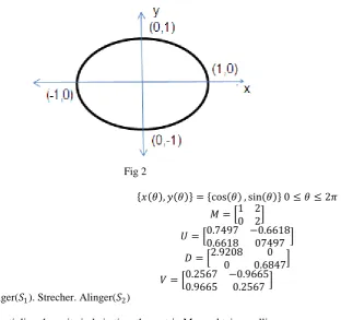
Fig 2

𝑥 𝜃 , 𝑦 𝜃 = cos 𝜃 , sin 𝜃 0 ≤ 𝜃 ≤ 2𝜋

𝑀 = 1 2_{0 2}

𝑈 = 0.7497 −0.6618_0.6618 ₀₇₄₉₇

𝐷 = 2.9208₀ _0.68470

𝑉 = 0.2567 −0.9665

0.9665 0.2567

M=hanger(𝑆1). Strecher. Alinger(𝑆2)

After mutipling the unit circle in time the matrix M we obtain an ellipse

Let 𝑀. 𝑥 𝜃 , 𝑦 𝜃

Fig 3

The product of aligned 𝑆2. {𝑥 𝜃 , 𝑦 𝜃 } is a circle

(4)

Which denote an over determined system of linear equation because𝑚 > 𝑛 And 𝑥𝑖, 𝑦𝑖 are given data 𝑎𝑖 are unknown

In the matrix form 𝐴𝑋 ≈ 𝑌

𝐴 = 1 ⋯ 𝑥1

𝑛−1

⋮ ⋱ ⋮

1 ⋯ 𝑥𝑚𝑛−1

𝑋 = 𝑎1 𝑎2 ⋮ 𝑎𝑛 𝑌 = 𝑦1 𝑦2 ⋮ 𝑦𝑚

∴ m- Equations with n unknown The residual vector is 𝑟 = 𝑌 − 𝐴𝑋

Using the Euclidean norms 𝑈 = 𝑚_𝑖=1𝑢_𝑖2 The least square problem becomes min𝐶 𝑌 − 𝐴𝑋 2

Let AX=Y

𝐴𝑇_{𝐴𝑋 = 𝐴}𝑇_𝑌

Which are known as the normal equation

The least square problem is obtained using SVD analysis of A as shown We have 𝐴 = 𝑈𝐷𝑉𝑇

𝑌 − 𝐴𝑋 2_{= 𝑌 − 𝑈𝐷𝑉𝑇 𝑋}2

= 𝑈𝑇 2_{𝑌 − 𝑈𝐷𝑉𝑇 𝑋}2

= 𝑈𝑇_{𝑌 − 𝐷𝑉𝑇𝑋}2

De𝑈𝑇𝑦 is D and 𝑉𝑇𝑋 and rank of A , we have 𝑌 − 𝐴 2= 𝑑𝐷𝑧 2=

𝑑1− 𝜎1𝑧1

𝑑2− 𝜎2𝑧2

⋮ 𝑑𝑟− 𝜎𝑟𝑧𝑟

= 𝑑1− 𝜎1𝑧1 2+ 𝑑2− 𝜎2𝑧2 2+ ⋯ + 𝑑𝑟− 𝜎𝑟𝑧𝑟 2

We can now uniquely solve𝑧𝑖 =𝑑_𝜎𝑖

𝑖 for 𝑖 = 1,2, … 𝑟

To reduce this expression to its minimum value, the solution to the least square is obtained for

𝑉𝑇_{𝑋 = 𝑍}

𝑋 = 𝑉𝑧

Examples

1. The population contain town is shown in the following table

Year 1920 1930 1940 1950 1960

Population 19.96 39.65 58.81 77.21 94.61

We want to fit a polynomial of degree 2 to these points. The polynomial is 𝑓 𝑥 = 𝑎0+ 𝑎1𝑥 + 𝑎2𝑥2

Such that 𝑓(𝑥𝑖) should be as close as possible to 𝑦𝑖 where the point 𝑥𝑖, 𝑦𝑖 ; 𝑖 = 1,2,3,4,5.

The year (𝑥𝑖) the population is (𝑦𝑖)

Our system of equation 𝐴𝑋 = 𝑌 is

1 1920 3686400

1 1930 37244900

1 1940 3763600

1 1950 3802500

1 1960 3841600

𝑎1 𝑎2 𝑎3 = 19.96 39.65 58.81 77.21 94.61

The SVD analysis of the matrix

(5)

𝑈𝑇_{𝑌 = −130.65 −57.18 −1.78}𝑇_{= 𝑑}

And compute 𝑧 = − 0.00000155 − 1.808 − 17903.842 𝑇Where 𝑧𝑖=𝑑_𝜎𝑖

𝑖, i=1,2,3.

𝑉𝑇_{𝑋 = 𝑧}

𝑋 = 𝑉𝑧

𝑋 = −17903.84 16.10 0.000000090555 𝑇

4. Conclusion

The singular value decomposition is nearly hundred years old.For the case of square matrices,it was discovered independently by Beltrami in 1873 and Jordan in 1874.

The technique was extended to rectangular matrices by Eckart and Young in the year 1930.

SVD of a matrix is still not widely used in education. This paper may useful for the further application of SVD.

5. References

[1] Alter, O., P. O. Brown, and D. Botstein. 2000. Singular value decomposition for genome-wide expression data processing and modeling. Proc. Natl. Acad. Sci. USA.97:10101–10106. [PMC free article][PubMed]

[2] Berman, H. M., J. Westbrook, Z. Feng, G. Gilliland, T. N. Bhat, H. Weissig, I. N. Shindyalov, and P. E. Bourne. 2000. The Protein Data Bank. Nucleic Acids Res.28:235–242. [PMC free article][PubMed]

[3] Borgstahl, G. E. O., D. R. Williams, and E. D. Getzoff. 1995. 1.4 Ångstrom structure of photoactive yellow protein, a cytosolic photoreceptor: unusual fold, active site, and chromophore. Biochemistry.34:6278–6287. [PubMed]

[4] D. Kahaner, C. Moler, S. Nash, Numerical Methods and Software, Prentice-Hall, Englewood Cliffs, NJ, 1989. [5] R.D. Skeel, J.B. Keiper, Elementary Numerical Computing with Mathematica, McGraw-Hill, New York, NY, 1993.