Importance Sampling for Minibatches

(1)

Importance Sampling for Minibatches

School of Mathematics University of Edinburgh Edinburgh, United Kingdom

Editor:Benjamin Recht

Abstract

Minibatching is a very well studied and highly popular technique in supervised learning, used by practitioners due to its ability to accelerate training through better utilization of parallel processing power and reduction of stochastic variance. Another popular technique is importance sampling—a strategy for preferential sampling of more important examples also capable of accelerating the training process. However, despite considerable effort by the community in these areas, and due to the inherent technical difficulty of the problem, there is virtually no existing work combining the power of importance sampling with the strength of minibatching. In this paper we propose the first practicalimportance sampling for minibatches and give simple and rigorous complexity analysis of its performance. We illustrate on synthetic problems that for training data of certain properties, our sampling can lead to several orders of magnitude improvement in training time. We then test the new sampling on several popular data sets, and show that the improvement can reach an order of magnitude.

keywords: empirical risk minimization; importance sampling; minibatching; variance-reduced methods; convex optimization

1. Introduction

Supervised learning is a widely adopted learning paradigm with important applications such as regression, classification and prediction. The most popular approach to training super-vised learning models is via empirical risk minimization (ERM). In ERM, the practitioner collects data composed of example-label pairs, and seeks to identify the best predictor by minimizing the empirical risk, i.e., the average risk associated with the predictor over the training data.

With ever increasing demand for accuracy of the predictors, largely due to successful industrial applications, and with ever more sophisticated models that need to be trained, such as deep neural networks Hinton (2007); Krizhevsky et al. (2012), or multiclass

classifi-∗. This author would like to acknowledge support from the EPSRC Grant EP/K02325X/1, Accelerated Coordinate Descent Methods for Big Data Optimization and the EPSRC Fellowship EP/N005538/1,

Randomized Algorithms for Extreme Convex Optimization.

c

(2)

cation Huang et al. (2012), increasing volumes of data are used in the training phase. This leads to huge and hence extremely computationally intensive ERM problems.

Batch algorithms—methods that need to look at all the data before taking a single step to update the predictor—have long been known to be prohibitively impractical to use. Typical examples of batch methods are gradient descent and classical quasi-Newton methods. One of the most popular algorithms for overcoming the deluge-of-data issue is stochastic gradient descent (SGD), which can be traced back to a seminal work of Robbins and Monro (1951). In SGD, a single random example is selected in each iteration, and the predictor is updated using the information obtained by computing the gradient of the loss function associated with this example. This leads to a much more fine-grained iterative process, but at the same time introduces considerable stochastic noise, which eventually— typically after one or a few passes over the data—effectively halts the progress of the method, rendering it unable to push the training error (empirical risk) to the realm of small values.

1.1 Strategies for dealing with stochastic noise

Several approaches have been proposed to deal with the issue of stochastic noise in the finite-data regime. The most important of these are i) decreasing stepsizes, ii) minibatching, iii) importance sampling and iv) variance reduction via “shift”, listed here from historically first to the most modern.

The first strategy, decreasing stepsizes, takes care of the noise issue by a gradual and

direct scale-down process, which ensures that SGD converges to the ERM optimum Zhang (2004). However, an unwelcome side effect of this is a considerable slowdown of the iterative process Bottou (2010). For instance, the convergence rate is sublinear even if the function to be minimized is strongly convex.

The second strategy, minibatching, deals with the noise by utilizing a random set of

examples in the estimate of the gradient, which effectively decreases the variance of the estimate Shalev-Shwartz et al. (2011). However, this has the unwelcome side-effect of re-quiring more computation. On the other hand, if a parallel processing machine is available, the computation can be done concurrently, which ultimately leads to speedup. This strategy does not result in an improvement of the convergence rate (unless progressively larger mini-batch sizes are used, at the cost of further computational burden Friedlander and Schmidt (2012)), but can lead to massive improvement of the leading constant, which ultimately

means acceleration (almost linear speedup for sparse data) Tak´aˇc et al. (2013).

The third strategy,importance sampling, operates by a careful data-driven design of the

probabilities of selecting examples in the iterative process, leading to a reduction of the variance of the stochastic gradient thus selected. Typically, the overhead associated with computing the sampling probabilities and with sampling from the resulting distribution is negligible, and hence the net effect is speedup. In terms of theory, for standard SGD this improves a non-dominant term in the complexity. On the other hand, when SGD is combined with variance reduction, then this strategy leads to the improvement of the leading constant in the complexity estimate, typically via replacing the maximum of certain

data-dependent quantities by their average Richtárik and Takáˇc (2016b); Koneˇcný et al. (2017);

Zhao and Zhang (2015); Qu et al. (2015); Needell et al. (2014); Csiba and Richt´arik (2015);

(3)

Finally, and most recently, there has been a considerable amount of research activity due to the ground-breaking realization that one can gain the benefits of SGD (cheap iterations) without having to pay through the side effects mentioned above (e.g., halt in convergence due to decreasing stepsizes or increase of workload due to the use of minibatches) in the finite data regime. The result, in theory, is that for strongly convex losses (for example), one does not have to suffer sublinear convergence any more, but instead a fast linear rate “kicks in”. In practice, these methods dramatically surpass all previous existing approaches.

The main algorithmic idea is to change the search direction itself, via a properly

de-signed and cheaply maintainable “variance-reducing shift” (control variate). Methods in

this category are of two types: those operating in the primal space (i.e., directly on ERM) and those operating in a dual space (i.e., with the dual of the ERM problem). Methods of the primal variety include SAG Schmidt et al. (2013), SVRG Johnson and Zhang (2013),

S2GD Koneˇcn´y and Richt´arik (2017), proxSVRG Xiao and Zhang (2014), SAGA Defazio

et al. (2014), mS2GD Koneˇcn´y et al. (2016) and MISO Mairal (2015). Methods of the dual

variety work by updating randomly selected dual variables, which correspond to examples. These methods include SCD Shalev-Shwartz and Tewari (2011), RCDM Nesterov (2012);

Richtárik and Takáˇc (2014), SDCA Shalev-Shwartz and Zhang (2013b), Hydra Richtárik

and Tak´aˇc (2016a); Fercoq et al. (2014), mSDCA Tak´aˇc et al. (2013), APCG Lin et al.

(2015), AsySPDC Liu and Wright (2015), RCD Necoara and Patrascu (2014), APPROX

Fercoq and Richt´arik (2015), SPDC Zhang and Xiao (2015), ProxSDCA Shalev-Shwartz

and Zhang (2012), ASDCA Shalev-Shwartz and Zhang (2013a), IProx-SDCA Zhao and Zhang (2015), and QUARTZ Qu et al. (2015).

1.2 Combining strategies

We wish to stress that the key strategies, mini-batching, importance sampling and variance-reducing shift, should be seen as orthogonal tricks, and as such they can be combined, achieving an amplification effect. For instance, the first primal variance-reduced method

allowing for mini-batching was Koneˇcn´y et al. (2016); while dual-based methods in this

cat-egory include Shalev-Shwartz and Zhang (2013a); Qu et al. (2015); Csiba and Richt´arik

(2015). Variance-reduced methods with importance sampling include Nesterov (2012);

Richtárik and Takáˇc (2014); Richtárik and Takáˇc (2016b); Qu and Richtárik (2016) for

gen-eral convex minimization problems, and Zhao and Zhang (2015); Qu et al. (2015); Needell

et al. (2014); Csiba and Richt´arik (2015) for ERM.

2. Contributions

Despite considerable effort of the machine learning and optimization research communities,

virtually no importance sampling for minibatches was previously proposed, nor analyzed.1.

The reason for this lies in the underlying theoretical and computational difficulties asso-ciated with the design and successful implementation of such a sampling. One needs to come up with a way to focus on a reasonable set of subsets (minibatches) of the examples to be used in each iteration (issue: there are many subsets; which ones to choose?),

(4)

sign meaningful data-dependent non-uniform probabilities to them (issue: how?), and then be able to sample these subsets according to the chosen distribution (issue: this could be computationally expensive).

The tools that would enable one to consider these questions did not exist until recently. However, due to a recent line of work on analyzing variance-reduced methods utilizing

what is known as arbitrary sampling Richt´arik and Tak´aˇc (2016b); Qu et al. (2015); Qu

and Richtárik (2016); Qu and Richtárik (2016); Csiba and Richtárik (2015), we are able

to ask these questions and provide answers. In this work we design a novel family of

samplings—bucket samplings—and a particular member of this family—importance

sam-pling for minibatches. We illustrate the power of this sampling in combination with the reduced-variance dfSDCA method for ERM. This method is a primal variant of SDCA,

first analyzed by Shalev-Shwartz (2015), and extended by Csiba and Richt´arik (2015) to

the arbitrary sampling setting. However, our sampling can be combined with any stochas-tic method for ERM, such as SGD or S2GD, and extends beyond the realm of ERM, to convex optimization problems in general. However, for simplicity, we do not discuss these extensions in this work.

We analyze the performance of the new sampling theoretically, and by inspecting the results we are able to comment on when can one expect to be able to benefit from it. We il-lustrate on synthetic data sets with varying distributions of example sizes that our approach

can lead todramatic speedupswhen compared against standard (uniform) minibatching, of

one or more degrees of magnitude. We then test our method on real data sets and confirm that the use of importance minibatching leads to up to an order of magnitude speedup. Based on our experiments and theory, we predict that for real data with particular shapes and distributions of example sizes, importance sampling for minibatches will operate in a favourable regime, and can lead to speedup higher than one order of magnitude.

2.1 Related work

The idea of using non-uniform sampling in the parallel regime is by no means new. In the following we highlight several recent approaches in a chronological order and we describe their main differences to our method.

The first attempt for a potential speed-up using a non-uniform parallel sampling was

proposed in Richt´arik and Tak´aˇc (2016b). However, to compute the optimal probability

vector one has to solve a linear programming problem, which can easily be more complex than the original problem. The authors do not propose a practical version, which would overcome this issue.

The approach described in Zhao and Zhang (2014) uses the idea of a stratified sampling, which is a well-known strategy in statistics. The authors use clustering to group the exam-ples into several partitions and sample an example from each of the partitions uniformly. This approach is similar to ours, with two main differences: i) we do not need clustering for our approach (it can be computationally very expensive) ii) we allow non-uniform sampling inside each of the partitions, which leads to the main speed-up in our work.

Instead of directly improving the convergence rate of the methods, the authors in Csiba

and Richt´arik (2015) propose a strategy to improve the synchronized parallel

(5)

groups, which have similar sum of the amount of nonzero entries. When each core processes a single group, it should take the same time to finish as all the other groups, which leads to shorter waiting time in synchronization. Although this is a non-uniform parallel sampling, this approach takes a completely different direction than our method. The only speedup of the method proposed in the above work is achieved due to a shorter waiting time during the synchronization between parallel processing units, while the method proposed in this work directly decreases the iteration complexity.

Lastly, in Harikandeh et al. (2015) the authors actually propose a scheme for importance sampling with minibatches. In the paper they assume, that they can sample a minibatch with a fixed size (without repetition), such that the probabilities of sampling individual examples will be proportional to some given values. However, this is easier said than done— until our work there was no sampling scheme, which would allow for such minibatches. Therefore, the authors theoretically described an idea, which can be used in practice using our scheme.

3. The Problem

LetX∈_Rd×n _{be a data matrix in which features are represented in rows and examples in}

columns, and lety∈_Rn _{be a vector of labels corresponding to the examples. Our goal is to}

find a linear predictorw∈Rdsuch thatx>i w∼yi, where the pairxi, yi ∈Rd×Ris sampled

from the underlying distribution over data-label pairs. In the L2-regularized Empirical Risk

Minimization problem, we find wby solving the optimization problem

min

w∈_Rd

"

P(w) := 1

n n

X

i=1

φi(X>:iw) +

λ

2kwk

2 2 #

, (1)

whereφi :R→Ris a loss function associated with example-label pair (X:i, yi), andλ >0.

For instance, the square loss function is given by φi(t) = 0.5(t−yi)2. Our results are

not limited to L2-regularized problems though: an arbitrary strongly convex regularizer can be used instead Qu et al. (2015). We shall assume throughout that the loss functions

are convex and 1/γ-smooth, where γ > 0. The latter means that for all x, y ∈ R and all

i∈[n] :={1,2, . . . , n}, we have

|φ0_i(x)−φ0_i(y)| ≤ 1

γ|x−y|.

This setup includes ridge and logistic regression, smoothed hinge loss, and many other problems as special cases Shalev-Shwartz and Zhang (2013b). Again, our sampling can be adapted to settings with non-smooth losses, such as the hinge loss.

4. The Algorithm

In this paper we illustrate the power of our new sampling in tandem with Algorithm 1 (dfSDCA) for solving (1).

The method has two parameters. A “sampling” ˆS, which is a random set-valued mapping

(6)

Algorithm 1 dfSDCA Csiba and Richt´arik (2015)

Parameters: Sampling ˆS, stepsize θ >0

Initialization: Choose α(0) ∈_Rn_,

set w(0) = _λn1 Pn

i=1X:iα(0)i , pi =Prob(i∈Sˆ)

for t≥1 do

Sample a fresh random setSt according to ˆS

fori∈St do

∆i=φ0i(X>:iw(t−1)) +α

(t−1)

i

α_i(t)=α_i(t−1)−θp−1_i ∆i

end for

w(t) =w(t−1)−P

i∈Stθ(nλpi)

−1_∆

iX:i

end for

assumptions are made on the distribution of ˆS apart from requiring that pi is positive for

each i, which simply means that each example has to have a chance of being picked. The

second parameter is a stepsizeθ, which should be as large as possible, but not larger than a

certain theoretically allowable maximum depending onP and ˆS, beyond which the method

could diverge.

Algorithm 1 maintains n “dual” variables, α(₁t), . . . , α(nt) ∈ R, which act as

variance-reduction shifts. This is most easily seen in the case when we assume that St = {i} (no

minibatching). Indeed, in that case we have

w(t)=w(t−1)− θ

nλpi

(g(_it−1)+X:iα(t

−1)

i ),

whereg_i(t−1) :=X:i∆i is the stochastic gradient. Ifθis set to a proper value, as we shall see

next, then it turns out that for alli∈[n],αi is convergingα∗i :=−φ0i(X>:iw∗), where w∗ is

the solution to (1), which means that the shifted stochastic gradient converges to zero. This means that its variance is progressively vanishing, and hence no additional strategies, such as decreasing stepsizes or minibatching are necessary to reduce the variance and stabilize the process. In general, dfSDCA in each step picks a random subset of the examples, denoted

asSt, updates variables αi(t) fori∈St, and then uses these to update the predictorw.

4.1 Complexity of dfSDCA

In order to state the theoretical properties of the method, we define

E(t):= λ

2kw

(t)₋_w∗_k2 2+

γ

2nkα

(t)₋_α∗_k2 2.

Most crucially to this paper, we assume the knowledge of parameters v1, . . . , vn > 0 for

which the following ESO2 inequality holds

E  

X

i∈St

hiX:i

2 ≤

n

X

i=1

pivih2i (2)

(7)

holds for all h ∈ _Rn_{. Tight and easily computable formulas for such parameters can be}

found in Qu and Richt´arik (2016). For instance, wheneverProb(|St| ≤ τ) = 1, inequality

(2) holds with vi = τkX:ik2. However, this is a conservative choice of the parameters.

Convergence of dfSDCA is described in the next theorem.

Theorem 1 (Csiba and Richt´arik (2015)) Assume that all loss functions{φi}are con-vex and 1/γ smooth. If we run Algorithm 1 with parameter θ satisfying the inequality

θ≤min

i

pinλγ

vi+nλγ

, (3)

where {vi} satisfy (2), then the potential E(t) decays exponentially to zero as

EhE(t)i≤e−θtE(0).

Moreover, if we set θ equal to the upper bound in (3) so that

1

θ = maxi

1

pi

+ vi

pinλγ

(4)

then

t≥ 1

θlog

(1 +λγ)E(0)

λγ

!

⇒ E[P(w(t))−P(w∗)]≤.

5. Bucket Sampling

We shall first explain the concept of “standard” importance sampling.

5.1 Standard importance sampling

Assume that ˆS always picks a single example only. In this case, (2) holds for vi =kX:ik2,

independently of p := (p1, . . . , pn) Qu and Richt´arik (2016). This allows us to choose the

sampling probabilities as pi ∼ vi +nλγ, which ensures that (4) is minimized. This is

importance sampling. The number of iterations of dfSDCA is in this case proportional to

1

θ(imp) :=n+ Pn

i=1vi

nλγ .

If uniform probabilities are used, the average in the above formula gets replaced by the maximum:

1

θ(unif) :=n+

maxivi

λγ .

Hence, one should expect the followingspeedupwhen comparing the importance and uniform

samplings:

σ:= maxikX:ik

2 1

n

Pn

i=1kX:ik2

. (5)

Ifσ = 10 for instance, then dfSDCA with importance sampling is 10×faster than dfSDCA

(8)

5.2 Uniform minibatch sampling

In machine learning, the term “minibatch” is virtually synonymous with a special sampling,

which we shall here refer to by the name τ-nice sampling Richt´arik and Tak´aˇc (2016).

Sampling ˆS isτ-nice if it picks uniformly at random from the collection of all subsets of [n]

of cardinality τ. Clearly,pi=τ /nand, moreover, it was show by Qu and Richt´arik (2016)

that (2) holds with {vi} defined by

v(_iτ-nice) =

d

X

j=1

1 +(|Jj| −1)(τ −1)

n−1

X2_ji, (6)

where Jj := {i ∈ [n] : Xji 6= 0}. In the case of τ-nice sampling we have the stepsize and

complexity given by

θ(τ-nice)= min

i

τ λγ

v_i(τ-nice)+nλγ

, (7)

1 θ(τ-nice) =

n

τ +

maxivi(τ-nice)

τ λγ . (8)

Learning from the difference between the uniform and importance sampling of single example (Section 5.1), one would ideally wish the importance minibatch sampling, which we are yet to define, to lead to complexity of the type (8), where the maximum is replaced by an average.

5.3 Bucket sampling: definition

We now propose a family of samplings, which we call bucket samplings. Let B1, . . . , Bτ be

a partition of [n] ={1,2, . . . , n} intoτ nonempty sets (“buckets”).

Definition 2 (Bucket sampling) We say that Sˆ is a bucket sampling if for all i ∈ [τ],

|Sˆ∩Bi|= 1 with probability 1.

Informally, a bucket sampling picks one example from each of the τ buckets, forming

a minibatch. Hence, |Sˆ| = τ and P

i∈Blpi = 1 for each l = 1,2. . . , τ, where, as before,

pi := Prob(i ∈ Sˆ). Notice that given the partition, the vector p = (p1, . . . , pn) uniquely

determines a bucket sampling. Hence, we have a family of samplings indexed by a single

n-dimensional vector. LetP_B be the set of all vectors p∈_Rn _{describing bucket samplings}

associated with partitionB ={B1, . . . , Bτ}. Clearly,

PB =

  

p∈Rn:

X

i∈Bl

pi= 1 for all l&pi ≥0 for alli

  

.

Note, that the sampling inside each bucket Bi can be performed in O(log|Bi|) time

using a binary tree, with an initial overhead and memory of O(|Bi|log|Bi|), as explained

(9)

5.4 Optimal bucket sampling

The optimal bucket sampling is that for which (4) is minimized, which leads to a complicated optimization problem:

min

p∈PB

max

i

1

pi

+ vi

pinλγ

subject to {vi}satisfy (2).

A particular difficulty here is the fact that the parameters{vi} depend on the vectorp in

a complicated way. In order to resolve this issue, we prove the following result.

Theorem 3 Let Sˆbe a bucket sampling described by partitionB ={B1, . . . , Bτ}and vector p. Then the ESO inequality (2) holds for parameters{vi} set to

vi =

d

X

j=1

1 +

1−_ω10

j

δj

X2_ji, (9)

where Jj :={i∈[n] : Xji6= 0}, δj :=Pi∈Jjpi andω

0

j :=|{l : Jj∩Bl 6=∅}|.

Observe thatJj is the set of examples which express featurej, andω0j is the number of

buckets intersecting with Jj. Clearly, that 1 ≤ ω0j ≤ τ (if ω0j = 0, we simply discard this

feature from our data as it is not needed). Note that the effect of the quantities{ω_j0}on the

value of vi is small. Indeed, unless we are in the extreme situation whenωj0 = 1, which has

the effect of neutralizingδj, the quantity 1−1/ω0j is between 1−1/2 and 1−1/τ. Hence,

for simplicity, we could instead use the slightly more conservative parameters:

vi =

d

X

j=1

1 +

1−1

τ

δj

X2_ji.

5.5 Uniform bucket sampling

Assume all buckets are of the same size: |Bl|= n/τ for all l. Further, assume that pi =

1/|Bl|=τ /n for all i. Then δj =τ|Jj|/n, and hence Theorem 3 says that

v_i(unif)=

d

X

j=1

1 + 1− 1

ω_j0

!

τ|Jj|

n

!

X2_ji, (10)

and in view of (4), the complexity of dfSDCA with this sampling becomes

1 θ(unif) =

n

τ +

maxivi(unif)

τ λγ . (11)

Formula (6) is very similar to the one for τ-nice sampling (10), despite the fact that the

sets/minibatches generated by the uniform bucket sampling have a special structure with

respect to the buckets. Indeed, it is easily seen that the difference between between 1 +τ|Jj|

n

and 1 +(τ−1)(|Jj|−1)

(n−1) is negligible. Moreover, if eitherτ = 1 or |Jj|= 1 for allj, thenω

0

j = 1

(10)

quantity \ iteration 1 2 3 4 5 6

maxi(|pnewi −poldi |) 7·10

−5 ₇_·₁₀−6 ₇_·₁₀−7 ₈_·₁₀−8 ₈_·₁₀−9 ₉_·₁₀−10

kpnew−poldk2 1·10−3 2·10−4 2·10−5 2·10−6 2·10−7 2·10−8

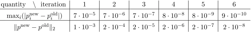
Table 1: Example of the convergence speed of the alternating optimization scheme forw8a

data set (see Table 5) with τ = 8. The table demonstrates the difference in

probabilities for two successive iterations (pold and pnew). We observed a similar

behaviour for all data sets and all choices ofτ.

6. Importance Minibatch Sampling

In the light of Theorem 3, we can formulate the problem of searching for the optimal bucket sampling as

min

p∈PB

max

i

1

pi

+ vi

pinλγ

subject to {vi}satisfy (9). (12)

Still, this is not an easy problem. Importance minibatch sampling arises as an

approx-imate solution of (12). Note that the uniform minibatch sampling is a feasible solution of the above problem, and hence we should be able to improve upon its performance.

6.1 Approach 1: alternating optimization

Given a probability distribution p ∈ PB, we can easily find v using Theorem 3. On the

other hand, for any fixedv, we can minimize (12) overp∈ PBby choosing the probabilities

in each groupBl and for each i∈Bl via

pi =

nλγ+vi

P

j∈Blnλγ+vj

. (13)

This leads to a natural alternating optimization strategy. An example of the standard convergence behaviour of this scheme is showed in Table 6.1. Empirically, this strategy

converges to a pair (p∗, v∗) for which (13) holds. Therefore, the resulting complexity will

be

1 θ(τ-imp) =

n

τ + maxl∈[τ]

τ n

P

i∈Blv

∗

i

τ λγ . (14)

We can compare this result against the complexity of τ-nice in (8). We can observe that

the terms are very similar, up to two differences. First, the importance minibatch sampling has a maximum over group averages instead of a maximum over everything, which leads

to speedup, other things equal. On the other hand, v(τ-nice) and v∗ are different quantities.

The alternating optimization procedure for computation of (v∗, p∗) is costly, as one iteration

(11)

6.2 Approach 2: practical formula

For each group Bl, let us choose for alli∈Bl the probabilities as follows:

p∗_i = nλγ+v

(unif)

i

P

k∈Blnλγ+v

(unif)

k

(15)

wherev_i(unif) is given by (10). Note that computing allv_i(unif) can be done by visiting every

non-zero entry of X once and and computing all p∗_i is a simple re-weighting. This is the

same computational cost as for standard serial importance sampling. Also, this process can

be straightforwardly parallelized, fully utilizing all the cores, which leads to τ times faster

computations. The overhead of using this sampling approach is therefore at most one pass over the data, which is negligible in most scenarios considered.

After doing some simplifications, the associated complexity result is

1

θ(τ-imp) = max_l (

n

τ +

τ n

P

i∈Blv

(unif)

i τ λγ

!

βl

)

, (16)

where

βl:= max

i∈Bl

nλγ+si

nλγ+v_i(unif), si:= d

X

j=1



1 + 1−

1

ω_j0

! X

k∈Jj

p∗_k

 X2_ji.

We would ideally want to haveβl= 1 for alll(this is what we get for importance sampling

without minibatches). If βl ≈1 for all l, then the complexity 1/θ(τ-imp) is an improvement

on the complexity of the uniform minibatch sampling since the maximum of group averages

is always better than the maximum of all elements v_i(uni):

n

τ +

maxl

τ n

P

i∈Blv

(unif)

i

τ λγ ≤

n

τ +

maxiv_i(unif)

τ λγ .

Indeed, the difference can be very large.

Finally, we would like to comment on the choice of the partitions B1, . . . , Bτ, as they

clearly affect the convergence rate. The optimal choice of the partitions is given by

minimiz-ing inB1, . . . , Bτ the maximum over group sums in (16), which is a complicated optimization

problem. Instead, we used random partitions of the same size in our experiments, which we believe is a good solution for the partitioning problem. The logic is simple: the minimum of the maximum over the group sums will be achieved, when all the group sums have similar values. If we set the partitions to the same size and we distribute the examples randomly, there is a good chance that the group sums will have similar values (especially for large amounts of data).

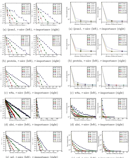
7. Experiments

We now comment on the results of our numerical experiments, with both synthetic and real

(12)

the test error (vertical axis) against the computational effort (horizontal axis). We measure

computational effort by the number of effective passes through the data divided by τ. We

divide byτ as a normalization factor; since we shall compare methods with a range of values

ofτ. This is reasonable as it simply indicates that theτ updates are performed in parallel.

Hence, what we plot is an implementation-independent model for time. We compared two algorithms:

1) τ-nice: dfSDCA using theτ-nice sampling with stepsizes given by (7) and (6),

2) τ-imp: dfSDCA usingτ-importance sampling (i.e., importance minibatch sampling)

defined in Subsection 6.2.

As the methods are randomized, we always plot the average over 5 runs. For each data set

we provide two plots. In the left figure we plot the convergence ofτ-nice for different values

of τ, and in the right figure we do the same for τ-importance. The horizontal axis has the

same range in both plots, so they are easily comparable. The values of τ we used to plot

areτ ∈ {1,2,4,8,16,32}. In all experiments we used the logistic loss: φi(z) = log(1 +e−yiz)

and set the regularizer toλ= maxikX:ik/n. We will observe the theoretical and empirical

ratio θ(τ-imp)/θ(τ-nice). The theoretical ratio is computed from the corresponding theory.

The empirical ratio is the ratio between the horizontal axis values at the moments when

the algorithms reached the precision 10−10.

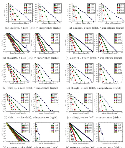
7.1 Artificial data

We start with experiments using artificial data, where we can control the sparsity pattern

of X and the distribution of {kX:ik2}. We fix n = 50,000 and choose d = 10,000 and

d= 1,000. For each feature we sampled a random sparsity coefficientω_i0 ∈[0,1] to have the

average sparsity ω0 := 1_dPd

i ω0i under control. We used two different regimes of sparsity:

ω0 = 0.1 (10% nonzeros) and ω0 = 0.8 (80% nonzeros). After deciding on the sparsity

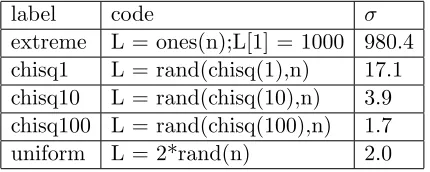
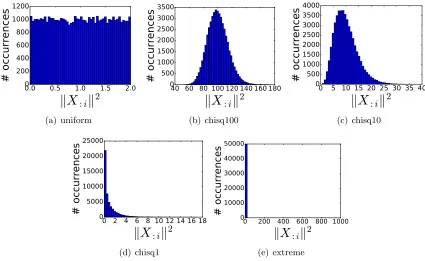
pattern, we rescaled the examples to match a specific distribution of norms Li = kX:ik2;

see Table 2. The code column shows the corresponding code in Julia to create the vector

of norms L. The distributions can be also observed as histograms in Figure 1.

label code σ

extreme L = ones(n);L[1] = 1000 980.4

chisq1 L = rand(chisq(1),n) 17.1

0 10000 20000 30000 40000 50000

# occurrences

(e) extreme

Figure 1: The distribution ofkX:ik2 for synthetic data

Data τ = 1 τ = 2 τ = 4 τ = 8 τ = 16 τ = 32

uniform 1.2 : 1.0 1.2 : 1.1 1.2 : 1.1 1.2 : 1.1 1.3 : 1.1 1.4 : 1.1

chisq100 1.5 : 1.3 1.5 : 1.3 1.5 : 1.4 1.6 : 1.4 1.6 : 1.4 1.6 : 1.4

chisq10 1.9 : 1.4 1.9 : 1.5 2.0 : 1.4 2.2 : 1.5 2.5 : 1.6 2.8 : 1.7

chisq1 1.9 : 1.4 2.0 : 1.4 2.2 : 1.5 2.5 : 1.6 3.1 : 1.6 4.2 : 1.7

extreme 8.8 : 4.8 9.6 : 6.6 11 : 6.4 14 : 6.4 20 : 6.9 32 : 6.1

Table 3: The theoretical : empirical ratios θ(τ-imp)/θ(τ-nice) for sparse artificial data

(ω0 = 0.1)

Data τ = 1 τ = 2 τ = 4 τ = 8 τ = 16 τ = 32

uniform 1.2 : 1.1 1.2 : 1.1 1.4 : 1.2 1.5 : 1.2 1.7 : 1.3 1.8 : 1.3

chisq100 1.5 : 1.3 1.6 : 1.4 1.6 : 1.5 1.7 : 1.5 1.7 : 1.6 1.7 : 1.6

chisq10 1.9 : 1.3 2.2 : 1.6 2.7 : 2.1 3.1 : 2.3 3.5 : 2.5 3.6 : 2.7

chisq1 1.9 : 1.3 2.6 : 1.8 3.7 : 2.3 5.6 : 2.9 7.9 : 3.2 10 : 3.9

extreme 8.8 : 5.0 15 : 7.8 27 : 12 50 : 16 91 : 21 154 : 28

Table 4: Thetheoretical:empiricalratiosθ(τ-imp)/θ(τ-nice). Artificial data withω0 = 0.8

(14)

7.2 Real data

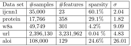
We used several publicly available data sets3, summarized in Table 5, which we randomly

split into a train (80%) and a test (20%) part. The test error is measured by the empirical risk (1) on the test data without a regularizer. The resulting test error was compared against the best achievable test error, which we computed by minimizing the corresponding risk. Experimental results are in Figure 7.3 and Figure 7.3. The theoretical and empirical speedup table for these data sets can be found in Table 6.

Data set #samples #features sparsity σ

ijcnn1 35,000 23 60.1% 2.04

protein 17,766 358 29.1% 1.82

w8a 49,749 301 4.2% 9.09

url 2,396,130 3,231,962 0.04 % 4.83

aloi 108,000 129 24.6% 26.01

Table 5: Summary of real data sets (σ = predicted speedup).

Data τ = 1 τ = 2 τ = 4 τ = 8 τ = 16 τ = 32

ijcnn1 1.2 : 1.1 1.4 : 1.1 1.6 : 1.3 1.9 : 1.6 2.2 : 1.6 2.3 : 1.8

protein 1.3 : 1.2 1.4 : 1.2 1.5 : 1.4 1.7 : 1.4 1.8 : 1.5 1.9 : 1.5

w8a 2.8 : 2.0 2.9 : 1.9 2.9 : 1.9 3.0 : 1.9 3.0 : 1.8 3.0 : 1.8

url 3.0 : 2.3 2.6 : 2.1 2.0 : 1.8 1.7 : 1.6 1.8 : 1.6 1.8 : 1.7

aloi 13 : 7.8 12 : 8.0 11 : 7.7 9.9 : 7.4 9.3 : 7.0 8.8 : 6.7

Table 6: The theoretical :empiricalratios θ(τ-imp)/θ(τ-nice).

7.3 Conclusion

In all experiments, τ-importance sampling performs significantly better than τ-nice

sam-pling. The theoretical speedup factor computed by θ(τ-imp)_/θ(τ-nice) _{provides an excellent}

estimate of the actual speedup. We can observe that on denser data the speedup is higher

than on sparse data. This matches the theoretical intuition forvi for both samplings.

Sim-ilar behaviour can be also observed for the test error, which is pleasing. As we observed for artificial data, for extreme data sets the speedup can be arbitrary large, even several orders

of magnitude. A rule of thumb: if one has data with large σ, practical speedup from using

importance minibatch sampling will likely be dramatic.

(15)

0 5 10 15 20

Number of Effective Passes / τ

1010-10

-9 10-8 10-7 10-6 10-5 10-4 10-3 10-2 10-1 P ( w

t)−

P ( w ∗) 1-nice 2-nice 4-nice 8-nice 16-nice 32-nice

0 5 10 15 20

1010-10 -9 10-8 10-7 10-6 10-5 10-4 10-3 10-2 10-1 P ( w

t)−

P ( w ∗) 1-imp 2-imp 4-imp 8-imp 16-imp 32-imp

(a) ijcnn1,τ-nice (left),τ-importance (right)

0 5 10 15 20 25 30

1010-10 -9 10-8 10-7 10-6 10-5 10-4 10-3 10-2 10-1 P ( w

t)−

0 5 10 15 20 25 30

1010-10

-9 10-8 10-7 10-6 10-5 10-4 10-3 10-2 10-1 P ( w

t)−

(b) protein,τ-nice (left),τ-importance (right)

0 5 10 15 20 25 30 35

1010-10

-9 10-8 10-7 10-6 10-5 10-4 10-3 10-2 10-1 P ( w

t)−

0 5 10 15 20 25 30 35

1010-10 -9 10-8 10-7 10-6 10-5 10-4 10-3 10-2 10-1 P ( w

t)−

(c) w8a,τ-nice (left),τ-importance (right)

0 50 100 150 200

10-10 10-9 10-8 10-7 10-6 10-5 10-4 10-3 10-2 P ( w

t)−

0 50 100 150 200

10-10 10-9 10-8 10-7 10-6 10-5 10-4 10-3 10-2 P ( w

t)−

(d) aloi,τ-nice (left),τ-importance (right)

0 10 20 30 40 50 60

1010-10 -9 10-8 10-7 10-6 10-5 10-4 10-3 10-2 10-1 P ( w

t)−

0 10 20 30 40 50 60

1010-10 -9 10-8 10-7 10-6 10-5 10-4 10-3 10-2 10-1 P ( w

t)−

(e) url,τ-nice (left),τ-importance (right)

Figure 2: Train error over iterations for data sets from Table 5

0 1 2 3 4 5

Number of Effective Passes / τ 10-2 10-1 Test suboptimality 1-nice 2-nice 4-nice 8-nice 16-nice 32-nice

0 1 2 3 4 5

Number of Effective Passes / τ 10-2 10-1 Test suboptimality 1-imp 2-imp 4-imp 8-imp 16-imp 32-imp

(a) ijcnn1,τ-nice (left),τ-importance (right)

0 1 2 3 4 5

Number of Effective Passes / τ 10-1 Test suboptimality 1-nice 2-nice 4-nice 8-nice 16-nice 32-nice

0 1 2 3 4 5

Number of Effective Passes / τ 10-1 Test suboptimality 1-imp 2-imp 4-imp 8-imp 16-imp 32-imp

(b) protein,τ-nice (left),τ-importance (right)

0 1 2 3 4 5 6 7

Number of Effective Passes / τ 10-2 10-1 Test suboptimality 1-nice 2-nice 4-nice 8-nice 16-nice 32-nice

0 1 2 3 4 5 6 7

Number of Effective Passes / τ 10-2 10-1 Test suboptimality 1-imp 2-imp 4-imp 8-imp 16-imp 32-imp

(c) w8a,τ-nice (left),τ-importance (right)

0 10 20 30 40 50 60

10-3 10-2 Test suboptimality 1-nice 2-nice 4-nice 8-nice 16-nice 32-nice

0 10 20 30 40 50 60

10-3 10-2 Test suboptimality 1-imp 2-imp 4-imp 8-imp 16-imp 32-imp

(d) aloi,τ-nice (left),τ-importance (right)

0 5_{Number of Effective Passes /}10 15 20 25 30 35 τ 10-4 10-3 10-2 10-1 Test suboptimality 1-nice 2-nice 4-nice 8-nice 16-nice 32-nice

0 5_{Number of Effective Passes /}10 15 20 25 30 35 τ 10-4 10-3 10-2 10-1 Test suboptimality 1-imp 2-imp 4-imp 8-imp 16-imp 32-imp

(e) url,τ-nice (left),τ-importance (right)

(16)

0 5 10 15 20

10-10 10-9 10-8 10-7 10-6 10-5 10-4 10-3 10-2 P ( w

t)−

0 5 10 15 20

10-10 10-9 10-8 10-7 10-6 10-5 10-4 10-3 10-2 P ( w

t)−

(a) uniform,τ-nice (left),τ-importance (right)

0 10 20 30 40 50

10-10 10-9 10-8 10-7 10-6 10-5 10-4 10-3 P ( w

t)−

0 10 20 30 40 50

10-10 10-9 10-8 10-7 10-6 10-5 10-4 10-3 P ( w

t)−

(b) chisq100,τ-nice (left),τ-importance (right)

0 5 10 15 20 25 30

10-10 10-9 10-8 10-7 10-6 10-5 10-4 10-3 P ( w

t)−

0 5 10 15 20 25 30

10-10 10-9 10-8 10-7 10-6 10-5 10-4 10-3 P ( w

t)−

(c) chisq10,τ-nice (left),τ-importance (right)

0 5 10 15 20 25

10-10 10-9 10-8 10-7 10-6 10-5 10-4 10-3 P ( w

t)−

0 5 10 15 20 25

10-10 10-9 10-8 10-7 10-6 10-5 10-4 10-3 P ( w

t)−

(d) chisq1,τ-nice (left),τ-importance (right)

0 10 20 30 40 50 60 70

10-10 10-9 10-8 10-7 10-6 10-5 10-4 10-3 P ( w

t)−

0 10 20 30 40 50 60 70

10-10 10-9 10-8 10-7 10-6 10-5 10-4 10-3 P ( w

t)−

(e) extreme,τ-nice (left),τ-importance (right)

Figure 4: Artificial data sets from Table 2

withω= 0.8

0 5 10 15 20

10-10 10-9 10-8 10-7 10-6 10-5 10-4 10-3 10-2 P ( w

t)−

0 5 10 15 20

10-10 10-9 10-8 10-7 10-6 10-5 10-4 10-3 10-2 P ( w

t)−

(a) uniform,τ-nice (left),τ-importance (right)

0 10 20 30 40 50

1010-10

-9 10-8 10-7 10-6 10-5 10-4 10-3 10-2 P ( w

t)−

0 10 20 30 40 50

1010-10 -9 10-8 10-7 10-6 10-5 10-4 10-3 10-2 P ( w

t)−

(b) chisq100,τ-nice (left),τ-importance (right)

0 5 10 15 20 25 30

10-10 10-9 10-8 10-7 10-6 10-5 10-4 10-3 10-2 P ( w

t)−

0 5 10 15 20 25 30

10-10 10-9 10-8 10-7 10-6 10-5 10-4 10-3 10-2 P ( w

t)−

(c) chisq10,τ-nice (left),τ-importance (right)

0 5 10 15 20 25

10-10 10-9 10-8 10-7 10-6 10-5 10-4 10-3 10-2 P ( w

t)−

0 5 10 15 20 25

10-10 10-9 10-8 10-7 10-6 10-5 10-4 10-3 10-2 P ( w

t)−

(d) chisq1,τ-nice (left),τ-importance (right)

0 10 20 30 40 50 60 70 80

10-10 10-9 10-8 10-7 10-6 10-5 10-4 10-3 P ( w

t)−

0 10 20 30 40 50 60 70 80

10-10 10-9 10-8 10-7 10-6 10-5 10-4 10-3 P ( w

t)−

(e) extreme,τ-nice (left),τ-importance (right)

Figure 5: Artificial data sets from Table 2

(17)

8. Proof of Theorem 3

8.1 Three lemmas

We first establish three lemmas, and then proceed with the proof of the main theorem. With

each sampling ˆS we associate an n×n “probability matrix” defined as follows: Pij( ˆS) =

Prob(i ∈ S, jˆ ∈ Sˆ). Our first lemma characterizes the probability matrix of the bucket

sampling.

Lemma 4 If Sˆ is a bucket sampling, then

P( ˆS) =pp>◦(E−B) + Diag(p), (17)

where E∈Rn×n is the matrix of all ones,

B:=

τ

X

l=1

P(Bl), (18)

and ◦ denotes the Hadamard (elementwise) product of matrices. Note that B is the 0-1 matrix given by Bij = 1 if and only if i, j belong to the same bucket Bl for some l.

Proof Let P=P( ˆS). By definition

Pij =

    

pi i=j

pipj i∈Bl, j ∈Bk, l6=k

0 otherwise.

It only remains to compare this to (17).

Lemma 5 Let J be a nonempty subset of [n], let B be as in Lemma 4 and put ω0_J :=|{l: J∩Bl6=∅}|. Then

P(J)◦B 1

ω0_JP(J). (19)

Proof For any h∈_Rn_{, we have}

h>P(J)h= X

i∈J

hi

!2

=

 

τ

X

l=1

X

i∈J∩Bl

hi

  2

≤ω_J0 τ

X

l=1

 

X

i∈J∩Bl

hi

  2

=ω_J0

τ

X

l=1

h>P(J ∩Bl)h,

where we used the Cauchy-Schwarz inequality. Using this, we obtain

P(J)◦B(18)= P(J)◦

τ

X

l=1

P(Bl) = τ

X

l=1

P(J)◦P(Bl) = τ

X

l=1

P(J ∩Bl)

(8.1)

1

(18)

Lemma 6 Let J be any nonempty subset of [n]and Sˆ be a bucket sampling. Then

P(J)◦pp> X

i∈J

pi

!

Diag(P(J∩Sˆ)). (20)

Proof Choose any h∈_Rn _{and note that}

h>(P(J)◦pp>)h= X

i∈J

pihi

!2

= X

i∈J

xiyi

!2

,

wherexi=

√

pihi and yi =

√

pi. It remains to apply the Cauchy-Schwarz inequality:

X

i∈J

xiyi ≤

X

i∈J

x2_i X

i∈J

y_i2

and notice that thei-th element on the diagonal ofP(J∩Sˆ) ispi fori∈J and 0 fori /∈J

8.2 Proof of Theorem 3

By Theorem 5.2 in Qu and Richt´arik (2016), we know that inequality (2) holds for

param-eters{vi} set to

vi =

d

X

j=1

λ0(P(Jj∩Sˆ))X2ji,

whereλ0(M) is the largest normalized eigenvalue of symmetric matrix Mdefined as

λ0(M) := max

h

n

h>Mh : h>Diag(M)h≤1o.

Furthermore,

P(Jj∩Sˆ) =P(Jj)◦P( ˆS)

(17)

= P(Jj)◦pp>−P(Jj)◦pp>◦B+P(Jj)◦Diag(p)

(19)

1− 1

ω_J0

P(Jj)◦pp>+P(Jj)◦Diag(p)

(20)

1− 1

ω_J0

δjDiag(P(Jj ∩Sˆ)) + Diag(P(Jj∩Sˆ)),

(19)

References

L´eon Bottou. Large-scale machine learning with stochastic gradient descent. In

COMP-STAT, pages 177–186. Springer, 2010.

Dominik Csiba and Peter Richt´arik. Primal method for ERM with flexible mini-batching

schemes and non-convex losses. arXiv:1506.02227, 2015.

Dominik Csiba, Zheng Qu, and Peter Richt´arik. Stochastic dual coordinate ascent with

adaptive probabilities. ICML, 2015.

Aaron Defazio, Francis Bach, and Simon Lacoste-Julien. Saga: A fast incremental gradient

method with support for non-strongly convex composite objectives. In NIPS 27, pages

1646–1654, 2014.

Olivier Fercoq and Peter Richt´arik. Accelerated, parallel, and proximal coordinate descent.

SIAM Journal on Optimization, 25(4):1997–2023, 2015.

Olivier Fercoq, Zheng Qu, Peter Richt´arik, and Martin Tak´aˇc. Fast distributed coordinate

descent for minimizing non-strongly convex losses. IEEE International Workshop on

Machine Learning for Signal Processing, 2014.

Michael P Friedlander and Mark Schmidt. Hybrid deterministic-stochastic methods for data

fitting. SIAM Journal on Scientific Computing, 34(3):A1380–A1405, 2012.

Reza Harikandeh, Mohamed Osama Ahmed, Alim Virani, Mark Schmidt, Jakub Koneˇcn´y,

and Scott Sallinen. Stop wasting my gradients: Practical SVRG. In NIPS 28, pages

2251–2259, 2015.

Geoffrey E Hinton. Learning multiple layers of representation. Trends in cognitive sciences,

11(10):428–434, 2007.

Guang-Bin Huang, Hongming Zhou, Xiaojian Ding, and Rui Zhang. Extreme learning

machine for regression and multiclass classification. Systems, Man, and Cybernetics,

Part B: Cybernetics, IEEE Transactions on, 42(2):513–529, 2012.

Rie Johnson and Tong Zhang. Accelerating stochastic gradient descent using predictive

variance reduction. In NIPS 26, 2013.

Jakub Koneˇcn´y and Peter Richt´arik. S2GD: Semi-stochastic gradient descent methods.

Frontiers in Applied Mathematics and Statistics, 3(9):1–14, 2017.

Jakub Koneˇcný, Jie Lu, Peter Richtárik, and Martin Takáˇc. mS2GD: Mini-batch

semi-stochastic gradient descent in the proximal setting. IEEE Journal of Selected Topics in

Signal Processing, 10(2):242–255, 2016.

Jakub Koneˇcn´y, Zheng Qu, and Peter Richt´arik. Semi-stochastic coordinate descent.

Op-timization Methods and Software, 32(5):993–1005, 2017.

Alex Krizhevsky, Ilya Sutskever, and Geoffrey E Hinton. Imagenet classification with deep

(20)

Qihang Lin, Zhaosong Lu, and Lin Xiao. An accelerated proximal coordinate gradient

method and its application to regularized empirical risk minimization. SIAM Journal on

Optimization, 25(4):2244–2273, 2015.

Ji Liu and Stephen J Wright. Asynchronous stochastic coordinate descent: Parallelism and

convergence properties. SIAM Journal on Optimization, 25(1):351–376, 2015.

Julien Mairal. Incremental majorization-minimization optimization with application to

large-scale machine learning. SIAM Journal on Optimization, 25(2):829–855, 2015.

Ion Necoara and Andrei Patrascu. A random coordinate descent algorithm for optimization

problems with composite objective function and linear coupled constraints.

Computa-tional Optimization and Applications, 57(2):307–337, 2014.

Deanna Needell, Rachel Ward, and Nati Srebro. Stochastic gradient descent, weighted

sampling, and the randomized kaczmarz algorithm. In NIPS 27, pages 1017–1025, 2014.

Yurii Nesterov. Efficiency of coordinate descent methods on huge-scale optimization

prob-lems. SIAM Journal on Optimization, 22(2):341–362, 2012.

Zheng Qu and Peter Richt´arik. Coordinate descent methods with arbitrary sampling I:

algorithms and complexity. Optimization Methods and Software, 31(5):829–857, 2016.

Zheng Qu and Peter Richt´arik. Coordinate descent with arbitrary sampling II: expected

separable overapproximation. Optimization Methods and Software, 31(5):858–884, 2016.

Zheng Qu, Peter Richt´arik, and Tong Zhang. Quartz: Randomized dual coordinate ascent

with arbitrary sampling. In NIPS 28, pages 865–873, 2015.

Peter Richt´arik and Martin Tak´aˇc. Distributed coordinate descent method for learning with

big data. JMLR, 17(75):1–25, 2016a.

Peter Richt´arik and Martin Tak´aˇc. On optimal probabilities in stochastic coordinate descent

methods. Optimization Letters, 10(6):1233–1243, 2016b.

Peter Richt´arik and Martin Tak´aˇc. Iteration complexity of randomized block-coordinate

descent methods for minimizing a composite function. Mathematical Programming, 144

(2):1–38, 2014.

Peter Richt´arik and Martin Tak´aˇc. Parallel coordinate descent methods for big data

opti-mization. Mathematical Programming, 156(1):433–484, 2016.

Herbert Robbins and Sutton Monro. A stochastic approximation method. Ann. Math.

Statist., 22(3):400–407, 1951.

Mark Schmidt, Nicolas Le Roux, and Francis Bach. Minimizing finite sums with the

stochas-tic average gradient. arXiv:1309.2388, 2013.

(21)

Shai Shalev-Shwartz and Ambuj Tewari. Stochastic methods for `1-regularized loss

mini-mization. JMLR, 12:1865–1892, 2011.

Shai Shalev-Shwartz and Tong Zhang. Proximal stochastic dual coordinate ascent.

arXiv:1211.2717, 2012.

Shai Shalev-Shwartz and Tong Zhang. Accelerated mini-batch stochastic dual coordinate

ascent. In NIPS 26, pages 378–385. 2013a.

Shai Shalev-Shwartz and Tong Zhang. Stochastic dual coordinate ascent methods for

reg-ularized loss. JMLR, 14(1):567–599, 2013b.

Shai Shalev-Shwartz, Yoram Singer, Nathan Srebro, and Andrew Cotter. Pegasos: Primal

estimated sub-gradient solver for svm. Mathematical Programming, 127(1):3–30, 2011.

Martin Tak´aˇc, Avleen Singh Bijral, Peter Richt´arik, and Nathan Srebro. Mini-batch primal

and dual methods for SVMs. In ICML, 2013.

Lin Xiao and Tong Zhang. A proximal stochastic gradient method with progressive variance

reduction. SIAM Journal on Optimization, 24(4):2057–2075, 2014.

Tong Zhang. Solving large scale linear prediction problems using stochastic gradient descent

algorithms. In ICML, 2004.

Yuchen Zhang and Lin Xiao. Stochastic primal-dual coordinate method for regularized

empirical risk minimization. In ICML, 2015.

Peilin Zhao and Tong Zhang. Accelerating minibatch stochastic gradient descent using

stratified sampling. arXiv:1405.3080, 2014.

Peilin Zhao and Tong Zhang. Stochastic optimization with importance sampling. InICML,