Vol. 32, No. 1, March, 2013, pp. 81–92. Copyright©2013 Faculty of Engineering, University of Nigeria. ISSN 1115-8443
MINIMUM VARIANCE ESTIMATION OF YIELD
PARAMETERS OF RUBBER TREE WITH KALMAN FILTER
A.C. Igboanugoa,U.E. Ucheb
Department of Production Engineering, Faculty of Engineering, University of Benin, Benin-City, Nigeria.
Emails: a[email protected];b[email protected]
Abstract
Although growth and yield data are available in rubber plantations in Nigeria for aggregate rubber production planning, existing models poorly estimate the yield per rubber tree for the incoming year. Kalman filter, a flexible statistical estimator, is used to combine the inexact prediction of the rubber production with an equally inexact rubber yield, tree girth, tapping height, stimulation and tapping system measurements to obtain an optimal estimate of one year ahead rubber production. Six rubber clones-GT1, PB260, PB217, PB28/59, PB324 and RRIM703 were studied using 12-year data, generated from permanent experimental plots. Stochastic autoregressive model was fitted to the data to identify optimal management strategy that accounts for risk due to seasonality. STAMP, an OxMetric modular software system for time series analysis, was used to estimate the yield parameters. Our results show that significant test of actual yield to model forecast is less than 1.96. Hence, the null hypothesis that the actual yield is within the forecasted value is accepted at 5% significant level. Based on the impulse response function of the lead equations, the long-run elasticity of yield was estimated to be highest for PB324 (2211gm/tree) and lowest for RRIM703 (1053gm/tree). PB260 is the best short term clone with the highest dynamic multiplier of 0.59. More important, the estimator minimized the variance of estimation errors from 55% of plantation prevision to 10%. It is our opinion that Kalman filter is a robust estimator of the biotechnical dynamics of rubber exploitation system.
Keywords: Kalman filter, parameter estimation, rubber clones, Chow failure test, autocorrelation, STAMP, data characterization
1. Introduction
Obtaining reliable information for the predictive yield of rubber clones that is needed for aggregate rubber production planning and for the determination of the long run elasticity of yield, required for rub-ber clone selection from historical yield and growth data, has remained a great challenge for rubber plan-tation managers: the information emanating therein is found to be replete with imprecision for purposes of planning due to substantial error in measurements, heterogeneity of plants population in age and size, non independence of observations and multiple obser-vations with serial correlation. The current predic-tion models which include use of mean [1], ratio [2] and the linear regression predictors [3] are considered rather inappropriate because several characteristics of the modelling data violate statistical assumptions un-derlying regression techniques. Further, the objective
2. Review of Literature
In this paper, the objective is to modify the popu-lation model to make a better prediction for a specific agricultural field not for a general situation. A filter is an algorithm that is applied to a time series to im-prove it in some way- filtering out noise. The task of filtering is to eliminate by some means as much of the noise as possible through processing of the measure-ments. This task is achieved by using measured values to update the model state variables each time an ob-servation is available. Hence, Kalman filter is not just a linear estimator where the slope (A) is a fixed matrix and the intercept (b) a fixed vector but it is a linear minimum variance estimator where the slope (A0) and
the intercept (b0) in the prediction equation are
cho-sen to minimize the expected mean square error such that[4]:
EkX−A0Y −b0k2≤EkX−AY −bk2∀A, b (1)
The basic key to this process is the structural time series state space model in which the state of the time series is represented by its various unobserved compo-nents such as trend and seasonality.
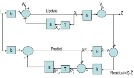
In using Kalman filter as an estimator, one of the in-dependent estimates is a current estimate or monitor-ing measurement and the other is a previous estimate that is updated for expected changes overtime using a prediction model (Fig. 1 refers.) The variance for the updated estimate includes the effects of the errors in the previous inventory that are propagated over time and the model prediction errors between previous and current estimates. Errors in the composite estimator are typically less than errors in either of the prior esti-mates alone [5]. The drawback of the Kalman filter is that it assumes that the model estimates are unbiased [6].The simple Kalman filter is therefore an optimal estimator, only if the system is linear and reasonable methods are available to accurately determine the co-variances P, Q, and R [7]. Further, when the normality assumption is dropped there is no longer any guaran-tee that the Kalman filter will give the conditional mean of the state vector though it remains an opti-mal estimator because it minimizes the mean square error within the class of all linear estimators [8].
The rubber tree yield model is treated as a time series in state-space form. The structure of the gen-eral state space models depends on the assumptions that are used to specify the state space vector com-ponents. In contrast to ARMA models, the specifi-cation of structural time series model requires judge-ments about the structures that are present in the sequence of observations. Following the presentation in [8] and [9], structural time series models consists of components that capture (deterministic or stochastic) trend, seasonality, and random error. Usingµtandβt to denote the trend and slope at time t, the relation
Figure 1: Kalman filter process.
between trend and slope is described as follows: Trend:
µt=µt−1+βt−1+ηt (2)
Slope:
βt=βt−1+ζt (3)
Seasonality:
s−1 X
j=0
γt−j =ωt (4)
System equation:
xt=φ1xt−1+φ2xt−2+. . .+φpxt−p+µt+γt+εt,
t=p+ 1. . . T
(5)
Substituting:
xt=φ1xt−1+. . .+φpxt−p+ (µt−1+βt−1+ηt)+
(ωt−γt−1−γt−2−. . .−γt−s+1) +εt
Measurement equation
zit=λixt+ξti i= 1,2, . . . , k, t= 1,2, . . . , T (6)
The equation is written in the form of the general state-space model with εt, ηt, ζt assumed indepen-dent, normally distributed random variable with zero mean and finite variance. Thus the parameters to be estimated in structural time series formulations are:
φ . . . φp, σε2, σε2, ση2, σζ2, σ2ω, λ1, . . . , λk,Σξ.
Kalman Filter Minimum Variance Estimation of Rubber Tree Yield Parameters
below.
Xt=
xt
xt−1
·
xt−p+1 µt
βt
γt
γt−1 γt−2
.. .
γt−s+2 =
φ1 φ2 · · · φp 1 1 −1 −1 · · · −1
1 0 · · · 0 0 0 0 0 · · · 0
· · · ·
0 0 · · · 0 0 0 0 0 · · · 0
1 1 0 1
−1 −1 · · · −1
1 0 · · · 0
0 1 · · · 0
..
. ... ... ...
0 0 · · · 0
xt−1 xt−2
·
xt−p
µt−1 βt−1 γt−1 γt−2 γt−3
.. .
γt−s+1 +
ηt+ωt+εt 0 · 0 ηt ςt ωt 0 0 .. . 0 (7) where: Xt; d×1 vector used to represent the yield state of the clone at the start of period t, Zt; k×1 vector used to represent the current yield,∅: AR
co-efficients,εt: random error terms,ω: seasonal random error,λ: measurement transition matrix,η: trend er-ror or irregularity,t: the lag.
The unknown variances and the components are es-timated by casting the model into state space form and employing the Kalman filter in which the vari-ances are obtained using the expectation maximiza-tion (EM) algorithm. The EM algorithm is a recursive method of obtaining maximum likelihood estimates of the unknown elements of the state and error sys-tem matrices of the state space form. Estimates of the component are then calculated using a smooth-ing procedure which first estimates the components recursively for t = 1, . . . , T and then runs a second “backward” recursion over t = T, , 1 to obtain the smoothed estimates[10]. Full details of the estima-tion procedure may be found in [11]. Autocorrelaestima-tion and partial autocorrelations functions are tradition-ally used for selecting between ARMA models but does not apply to time series models in state-space form [12].
3. Material and Method
Growth data were obtained from a trial plot located at Osse River, Ovie South West Local Government Area of Edo State, Nigeria, established since 1990 for the purpose of monitoring and analyzing the dynamics of rubber clones of rubber plantation belonging to Rubber Estate Nigeria Limited (RENL). The site is planted with different standard rubber clones for long term periodic observation. The rubber clones are GT1, PB260, PB217, PB28/59, PB324 and RRIM703. Data are collected on budding and planting success, girth, resistance to disease, evolution of tapping density and yield per clone and by replicate. Diameter measurements are made at 100cm height on 40 trees per clone per Fisher plots biannually.
Once a clone is of the right girth (50cm at 1m) and tapping density (40%) the clone is opened for tapping. The trunk circumference is thereafter measured using a measuring tape at 1.7 metre height previously marked with white paint. The production is weighed in replicate and expressed in gram per tree (g/t) and in kilogram per hectare (kg/ha). The trial has been opened since 1998 and tapped on S2D4 6d/7 tapping intensity. In other words, the tapping system used is the half spiral cut (S2) from tapping year one to nine and alternate quarter cut (S4) and half spiral cut thereon at fourth daily frequency (D4), six days tapping, followed by one day rest(6D/7). Hence trees are tapped 6 times per month. Ethrel 10% is routinely used to enhance production- 1 gram of stimulant is applied on 1 cm band of the tapping panel after dilution with water to 2.5, 3.3 or 5% concentrations depending on the clone. The stimulation frequencies are varied depending on the clone and the year of tapping. A fairly standard and consistent tapping policy was followed over the period under study. The aforementioned clones were used to determine yield response to girth, tapping height, tapping system, concentration and rounds of stimulation. The yield data used consist of daily data averaged per tree in gram and summed by quarter. Total quarterly dry rubber production per year provides adequate data for yield parameter estimation and for forecasting the seasonal breakdown of the incoming year rubber production per tree using Kalman filter. The one year-ahead estimate is used to prepare the aggregate rubber production plan for the plantation.
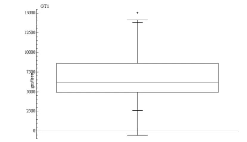
de-Figure 2: Box Plot of GT1 rubber yield data.
compose the series of 48 observed rubber yield values into unobserved trend and noise components. This is to facilitate the description of the series in terms of its component of interest such as the seasonal behaviour of yield and the trend movement. The predictive ca-pacity of the model is also enhanced by the decom-position. The stochastic trend model used here is the smooth trend in which the trend and its slope compo-nent evolve as random walk. The slope innovation and the noise component are assumed to be independent, zero mean white noises with constant variances.
The yield data analysis therefore involved selecting a model and fitting it to the generated data so as to estimate the parameters using Structural Time Series Analyser, Modeller and Predictor–STAMP software, which executes the process as described earlier. Fur-ther, the normal probability plots of the residual are obtained to support the result and assumptions on error terms. Finally, Kalman filter is applied to mini-mize the noise associated with the forecast of the time series model. In selecting between deterministic (risk free) and stochastic model, Akaikes Information Crite-rion (AIC) and Bayesian Information CriteCrite-rion (BIC) were used to measure the trade-off between predic-tion error and number of explanatory variables with smaller values being preferable:
AIC= −2×loglik+ 2×(n+d)
T (8)
BIC=−2×loglik+ log(T)×n (9)
where loglikis the logarithm of the model likelihood,
n is the number of estimated parameters and T is number of data.
The estimated parameters were subjected to signifi-cance analysis to decide which explanatory variable is important in determining the dynamic of the rubber production. Backward elimination was used to refine the model by removing the statistically insignificant parameters from the model specification. Further, the selected model was tested using prediction error vari-ance (p.e.v.) which is the basic measure of goodness of fit in time series model in the form of mean de-viation and Ljung-Box statistic, the Q statistics that measures lack of fit. In addition to this goodness of fit test, models are further diagnosed by generating in-sample and out-of sample predictions. In-sample predictions were made from t = d+ 1 to t = T
Kalman Filter Minimum Variance Estimation of Rubber Tree Yield Parameters
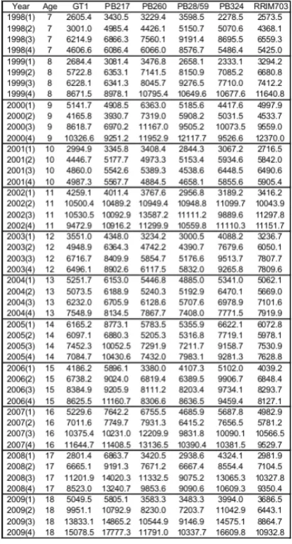
Table 1: 12-Year yield data of six RENL rubber clones (gm/tree).
matching the model to data. Hence solutions should be viewed with caution in that case.
4. Results and Discussion
4.1. Data characterization
Table 1 depicts the quarterly rubber production per tree from 1998 to 2009 for the six rubber clones under study. A box plot for the characterization of the GT1 rubber production data is shown in Figure 2, while Table 2 shows the result of data characterization of all the clones. Two clones GT1 and PB217 have out-liers due to change in stimulation from 2.5 to 5% for 2009 physiological year. The interquartile range of the rubber clones sample data ranges from 3708g for RRIM703 to 4525g for PB324 rubber clones. This ob-servation reflects the variability in the rubber clone yield response to seasonal changes. In other words, PB324 is more sensitive to season than RRIM703.
4.2. Plot inspection
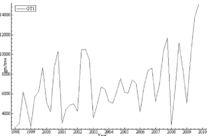
Figure 3 shows the actual plot of GT1 rubber clone yield per tree from January 1998 to December 2009. The graph shows a seasonal pattern of yield usually associated with tropical climate of dual seasons- dry and wet season within a year. The overall trend of the series is constant over the years. Its salient character-istics are a trend, which represents the long-run move-ments in the series, a seasonal pattern which repeats itself more or less every year and the irregular compo-nents which reflects non-systematic movement in the series. The choice of model is therefore informed by the decomposition of the series into its components as shown in Figure 4. The model to be considered initially is therefore the basic structural time series model (BSM) without cycle which is given by:
yt=µt+γt+εt (10)
whereµtis the local level component modelled as the random walk µt+1 =µt+ξt, yt is the trigonometric seasonal components andεtis a disturbance term with mean zero and varianceσ2ε.
As displayed in Figure 4, the seasonal effect hardly changes and is therefore considered fixed. The esti-mated level does pick up the underlying movement of the series and the estimated irregular is alright.
Structural time series model that separately models all the series components -seasonality, trend and ex-planatory variables was therefore implemented within the framework of state-space representation. The con-vergence of the yield model at steady state is strong for all clones.
4.3. Comparism of rubber yield models - de-terministic Vs stochastic models
In Table 3, two models are compared - determin-istic and stochastic structural time series models for purposes of model specification. Goodness of fit pa-rameters and prediction criteria used are shown in the table. From the table, the lead model is stochastic-lower Akaike information criterion (AIC), stochastic-lower Q-stat, higher Rs2 and better normality.
4.4. Parameter estimation
The result of the optimization algorithm in Table 4 is obtained from quarterly rubber yield per tree and the explanatory variable data set of the six RENL rub-ber clones under study as processed by STAMP. The series is modelled as a linear combination of trend, sea-sonal, irregular, autoregression and explanatory vari-ables (11).
Table 2: Box plot data characterization.
Clones Minimum Maximum 1st Ql* Median 3rd Qu* IQR* LW* UW* Outlier GT1 2605 15078 4882 6230 8623 3741 -730 14235 15078 PB217 3081 17777 5828 7406 10083 4255 -555 16466 17777 PB260 3229 13587 5031 6980 99467 4436 -1623 16121 -PB28/59 2658 12118 4736 6402 9133 4397 -1860 15729 -PB324 2279 16610 5377 7715 9902 4525 -1411 16690 -RRIM703 2574 12370 5014 6620 8722 3708 -548 14284 -*QL = Lower quartile, Qu = Upper quartile, IQR = Interquartile range, LW = Lower whisker, UW = Upper whisker
Table 3: Comparism of rubber yield deterministic and stochastic models.
Clones
Pev-D
Pev-S
Nor-D
Nor-S
H(12)-D
H(12)-S
Q-D Q-S Rs2
-D
Rs2 -S
AIC-D
AIC-S
Pev/ Md-D
Pev/ Md-S
GT1 1.91 1.87 2.84 1.75 0.98 1.27 7.7 5.6 0.61 0.62 14.93 14.9 1.09 1.14
PB217 2.02 1.97 6.75 4.4 0.74 0.81 6.3 7.4 0.57 0.58 14.97 14.95 1.04 1.01
PB260 2.68 2.45 6.78 2.73 0.39 0.67 25.2 16.61 0.54 0.58 15.26 15.17 1.01 1.17
PB28/59 1.96 1.99 5.84 7.06 0.14 0.19 15.3 18.1 0.59 0.59 14.95 14.96 1.18 1.38
PB324 1.93 1.88 1.56 6.01 0.67 0.60 10.3 8.33 0.62 0.62 14.93 14.91 1.35 1.11
R703 2.03 2.27 3.27 3.11 0.23 0.36 12.6 9.0 0.59 0.54 14.98 15.09 1.12 1.08
Table 4: Parameter estimation.
Clone Seasonal
σ2ω
Irregular
σ2ε
Level
σ2η
Slope
σ2ξ φ1
AR(1)
Lead Indicator -Ht
Lead Indicator -Gth
Lead Indi-cator Stim. Conc.
Lead Indi-cator Stim. Round GT1 0 115293 11659 0 0.39 25** 931*
PB217 0 1168 0 0 0.30 -553* 687**
PB260 0 0 0 2735 0.59 28** 531** PB28/59 0 0 0 1161 0.51 24** -856***
PB324 0 0 0 0 0.32 1570*** RRIM703 0 609 0 6078 0.33 -737**
***0.01, **0.05 and *0.1 significant level
Kalman Filter Minimum Variance Estimation of Rubber Tree Yield Parameters
Figure 4: RRIM 703 gm/tree decomposition of actual series (black) into level (broken), seasonal and irregular.
The model parameters are estimated by maximum likelihood (exact score). Autoregression and explana-tory variable coefficients estimated by STAMP are as shown in Table 4. The level of significance of each explanatory variable is depicted by *, ** and *** rep-resenting 0.1, 0.05 and 0.01 significant level of the co-efficient being zero i.e. of Tcritical > Tcalculated -accepting the null hypothesis of no significant contri-bution in the model. Hence any of the coefficients with probability below any of these figures is considered sig-nificant and forms part of the lead equation. Tapping system is found not to be important at all three levels of significance within the limits of analysed data set and period and therefore eliminated from further con-sideration as yield explanatory variable. Rubber yield and marginal girth increment are inversely related.
Multivariable models are used to improve the accu-racy of predictions [13].The coefficient of the explana-tory variables: - girth, tapping cut height, stimula-tion and stimulastimula-tion levels, tapping system, depicts the variables direct impact on yield per unit change in its value. It is worth noting that the estimated variance of disturbance for all the clones is zero except for GT1and PB217. This implies that the departure of the estimated trend from straight line as shown in Fig-ure 4 (level) is due to the effect of the explanatory vari-ables resulting from management exploitation policies on rubber tree stimulation, tapping cut height, clone selection, tapping system etc. The model estimates of negative girth relation to yield is supported by the var-ious literature reviewed earlier which have it that rub-ber production is in direct competition for metabolites with the biomass of the rubber tree [14] and [15]. This
observation underscores the ongoing trial in Nigeria on inorganic fertilizer supplemental application for rub-ber tree in tapping entitled “Interaction between Fer-tilization Levels of Rubber Tree Mature Crops and Yield Potential” - IFC-CIRAD-RENL Trial. Litera-ture also supports the inference on tapping cut height as it relates to increasing magnesium content of rubber tree with height for increase in latex production [16]. Seasonality that renders the rubber business risky and therefore stochastic is significant on the yield of all the clones at 99% confidence level and therefore is of high management interest as it defines the processing plant raw material supply chain and hence marketing plan. The result matches the wet and dry spell of southern Nigeria and its effect on rubber tree latex production. The seasonal value by quarter is estimated for each clone to be used for appropriate quarterly adjustment in the aggregate rubber production planning.
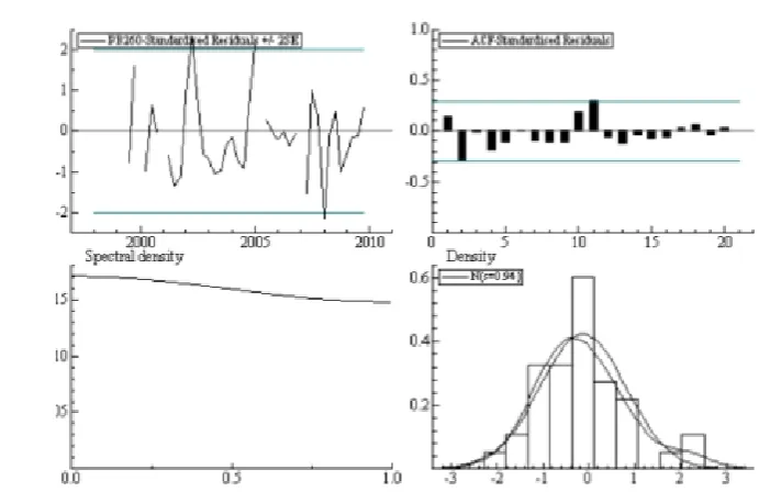
Figure 5: PB260 Residual statistics plot.
4.5. Long run elasticity of rubber yield per tree The long-run height elasticity of rubber production per tree is obtained from the lead equation of each rubber clone: xt= 0.39xt−1+25ht+931st+µt+γt+εt, εtvN(0, 1.2E+ 05) of GT1 rubber clone for instance as follows [18]:
lim j→∞
∂yt+j
∂wt
+ ∂yt+j
∂wt+1
+ ∂yt+1
∂wt+2
+· · ·+ ∂yt+j
∂wt+j
= 1 +φ+φ2+· · ·= 1/(1−φ)∀ ≤1 (12)
where wt = random variable and φ = the dynamic multiplier
25
1−0.39 = 41
The result suggests that a permanent 1cm increase in tapping height will lead to 41g increase in rubber production per tree. PB324 has the highest long run elasticity of yield of 2211 gm per tree while RRIM 703 has the least potential of 1053gm/tree on the long run as shown in Table 5.
4.6. Test of mis-specification
R2
s: The most suitable coefficient of determination is that around the season mean (Table 5) because of the seasonal effect, which for all the clones is positive and far from zero- greater than 50. Its relevance as a goodness of fit criterion is therefore not marginal. Normality: In Table 3.5, PB28/59 model normality is 7.06>5.99 at 5% critical value with 2 degree of free-dom. Hence the predictive value of PB28/59 model is highly suspect with the generated data. Higher nor-mality values are often caused by outliers.
Table 8: Chow failure test statistics.
Clones Failure Chi2 Test
P-value Accept Ho GT1 11.69 0.17 >0.05 PB217 11.81 0.16 >0.05 PB260 9.88 0.27 >0.05 PB28/59 3.27 0.92 >0.05 PB324 8.54 0.38 >0.05 RRIM703 4.21 0.83 >0.05
Q(q,d)-stat-The Box-Ljung Q-statistics is a test for residual serial correlation based on the first q resid-ual autocorrelations and distributed approximately as
χ2dwhere d=q−pis a lack of fit statistics. If model
captur-Kalman Filter Minimum Variance Estimation of Rubber Tree Yield Parameters
Table 5: Impulse response function and Long-run elasticity of yield/tree in grams.
Clones Dynamic mul-tiplier AR(1)
Height Impulse Re-sponse Function
Girth Impulse Re-sponse Function
Stimulation Impulse Response Function
Long-run elas-ticity of yield
PB324 0.32 1570 2211
PB217 0.30 -555 687 1774
PB28/59 0.51 24 -856 1600
GT1 0.39 25 931 1541
PB260 0.59 28 531 1118
RRIM703 0.33 -737 1053
Table 6: Test of mis-specification.
Clone Rs2 Q-Stat Q-Prob. Std Error Normality r(1) H(12)
Durbin-Watson GT1 0.62 5.61 0.40 1368 1.75 0.02 1.27 1.78 PB217 0.58 7.4 0.53 1404 4.4 0.05 0.81 1.80 PB260 0.58 16.6 0.06 1565 2.73 0.22 0.67 1.50 PB28/59 0.59 18.13 0.06 1410 7.06 0.21 0.19 1.56 PB324 0.62 8.33 0.21 1372 6.02 0.27 0.60 1.70 RRIM703 0.54 8.99 0.15 1506 3.11 0.16 0.36 1.59
Table 7: Test of specification result.
Clone Ratio p.e.v/m.d in square
Residual Skewness
Residual Kurtosis
Residual Bowman Shenton Ch2
p-value P<0.05 = S
GT1 1.14 0.43 0,18 1.24 0.54 NS PB217 1.01 0.73 0.15 3.41 0.18 NS PB260 1.16 0.57 0.43 2.36 0.31 NS PB28/59 1.39 1.01 1.9 11.92 0.003 S PB324 1.1 0.43 0.05 1.19 0.55 NS R703 1.08 0.64 0.16 2.63 0.27 NS
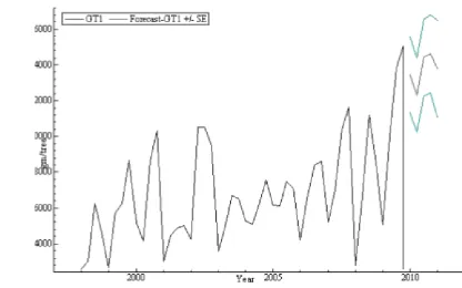
Figure 7: Kalman filter one-step ahead forecast of yield per tree for aggregate production planning.
ing the dynamic structure of the series. The r(1) is the serial correlation coefficients at the first lag (Ta-ble 6) distributed approximately as N(0,1/T) where T is the length of the time series. The acf fluctuates close to zero [r(1)] and fall within 95% confidence interval given by±1.96/√T±0.28 for large sample. Hence the model produced non significant residual autocorrela-tion.
Heteroskedasticity (H) occurs when the errors for different dates have different variances but are un-correlated with each other. H(h) is the ratio of the squares of the last h residuals to the squares of the first h residuals where h is set to the closest integer of T/3 [11]. A high value on F-distribution indicates an increase in variance overtime. A test for Heteroskedas-ticity distributed approximately as F (h,h) gives 2.69. The low value for the Heteroskedasticity statistic H (12) indicates a degree of Heteroskedasticity in the residuals which is however not significant (Table 6).
In summary, a strong evidence of first-order auto-correlation is established using Durbin-Watson test statistic for the six clones which cast doubt on any in-ferences drawn from a least squares model currently in use. Hence, a time series model that accounts for the autocorrelation of the random error was implemented in the study. Coefficient of determination Rs2, that
measures the percentage change in the series explained by the model, is that around the season mean. It is positive for all the clones and far from zero>50%. Its relevance as a goodness of fit criterion is therefore not marginal. The result of the residual autocorrelation
function (acf) test shows that the models explain the persistence by producing random residuals which sat-isfies the statistical assumption of the Kalman filter.
4.7. Residual test
Further, the assumptions underlying the local level model are that the disturbances εt and ηt are nor-mally distributed and serially independent with con-stant variances. The Normality: 5% null hypothe-sis of normality on Bowman-Shenton χ2 distribution
is shown in Table 7. PB28/59 residual is not nor-mally distributed with Bowman-Shenton χ2 p-value
at 0.003<0.05. Ratio p.e.v./m.d in square- The basic goodness of fit measure is the prediction error variance (PEV) whose square root is the equation standard er-ror. It is the variance of the residuals in the steady state. The ratio prediction error variance/mean de-viation square should be equal to unity for correctly specified model. In Table 7 the goodness of fit crite-rion is found satisfactory for five clones PB 217, GT1, PB260, PB324 and RRIM 703 with near unity but rather on the high side for PB 28/59 at 1.38. This out come will be useful in the post sample period evalua-tion of the models.
Kalman Filter Minimum Variance Estimation of Rubber Tree Yield Parameters
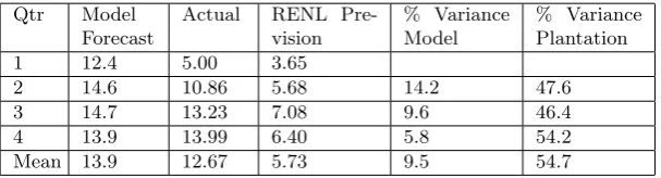
Table 9: Variance of model forecast to actual 2010 (kg/tree).
Qtr Model Forecast
Actual RENL Pre-vision
% Variance Model
% Variance Plantation 1 12.4 5.00 3.65
2 14.6 10.86 5.68 14.2 47.6 3 14.7 13.23 7.08 9.6 46.4 4 13.9 13.99 6.40 5.8 54.2 Mean 13.9 12.67 5.73 9.5 54.7
depicts the standardized residual plot, the autocorre-lation function and the cumulative sum residual plot. The standardized residual is the prediction error or innovation divided by the prediction error standard deviation while the cumulative sum is the sum of the residuals divided by the standard deviation. It is used to detect structural change in the model. The result of the residual acf plot shows that the models explain the persistence by producing random residuals which satisfies the statistical assumption of the Kalman filter (Fig 5).
4.8. In sample prediction test
Fig 6 shows the measured/calculated plotted against time as produced, in order to see how the model error varies with the dependent variable. The 8-quarter in-sample predictive test for RRIM703 shows that prediction and observed values fall within the in-tervals, confirming absence of any major intervention on the process. The prediction against observed val-ues (Fig 6) is to check the agreement between mea-sured and calculated values. The standardized plot is based on the residuals divided by the estimate of the standard deviation. The cumulative sum test is also plotted. The in-sample prediction is clearly consistent with structure of the model specification with predic-tion line plots falling within the specified intervals.
The Chow failure test probability at 95% confidence level is greater than 0.05 (p>0.05). The difference be-tween one step predictions and observations is there-fore not significant. Table 8 shows test result for all the clones on residuals.
4.9. Incoming year rubber production forecast Figure 7 shows the yield forecast of the incoming year. The lines on the either side of the forecast func-tion are based on the estimated root mean square er-ror (RMSE) and indicate the prediction interval that limits the rubber yield per tree estimate used for the aggregate production plan. As the forecast horizon increases so does the uncertainty attached to the fore-casts and the prediction interval becomes wider. The one year ahead forecast from Fig 7 is shown in Table 9 compared with actual 2010 production and RENL prevision for the same year. The gap between ac-tual rubber production and Kalman filter estimation
model is reduced to 10% on the average against plan-tation management prevision gap of 55%. First quar-ter 2010 is far from the predicted but in line with data trend and closer to RENL prevision. The increase in stimulation concentration from 2.5% to 5% is a pos-sible reason for the high model forecast value for the 1st quarter of 2010/11.
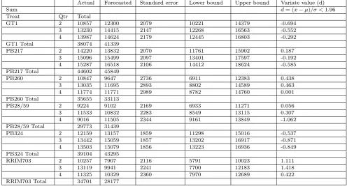
Significant test of actual yield to one year ahead model forecast in Table 10 is less than 1.96 for the rubber clones and hence the null hypothesis that the actual yield is within the forecasted value is accepted at 5% significant level (95% confidence level).
5. Conclusion
The structural time series decision models esti-mated by Kalman filtering provides an efficient an-alytical framework for tracking the yield dynamics of rubber plantations that results from various man-agement rubber exploitation policies. And guarded by theoretical insight, dependability of empirical data and judicious choice of analytical techniques, an ap-parently entrenched problem of noisy rubber crop col-lection and prediction environment has herein been rendered more predictable and dependable as a major contribution to rubber plantation industry. However, a wider application of the Kalman filter approach to rubber yield parameter estimation requires a deeper investigation of the Kalman filter assumptions, espe-cially the linearization of the rubber tree yield series, whose relaxation may render Kalman filter application heavy-going.
References
1. Ho, H., Chan Y., and Lim T. Environmax Plant-ing Recommendations- A New Concept in Choice of Clones. Proceedings of the Rubber Research Insti-tute of Malaysia Planters Conference, Kuala Lumpur, 1974, pp 293.
Table 10: Significant test of Actual Yield to Model Forecast.
Actual Forecasted Standard error Lower bound Upper bound Variate value (d)
Sum d= (x−µ)/σ <1.96
Treat Qtr Total
GT1 2 10857 12300 2079 10221 14379 -0.694
3 13230 14415 2147 12268 16563 -0.552
4 13987 14624 2179 12445 16803 -0.292
GT1 Total 38074 41339
PB217 2 14220 13832 2070 11761 15902 0.187
3 15096 15499 2097 13401 17597 -0.192
4 15287 16518 2106 14412 18624 -0.585
PB217 Total 44602 45849
PB260 2 10847 9647 2736 6911 12383 0.438
3 13035 11695 2893 8802 14589 0.463
4 11774 11771 2989 8782 14760 0.001
PB260 Total 35655 33113
PB28/59 2 9224 9102 2169 6933 11271 0.056
3 11533 10832 2283 8549 13115 0.307
4 9016 11505 2344 9161 13849 -1.062
PB28/59 Total 29773 31439
PB324 2 12159 13157 1859 11298 15016 -0.537
3 13442 15059 1857 13202 16917 -0.871
4 13503 15079 1856 13223 16936 -0.849
PB324 Total 39104 43295
RRIM703 2 10257 7907 2116 5791 10023 1.111
3 13119 9941 2241 7700 12183 1.418
4 11325 10329 2360 7970 12689 0.422
RRIM703 Total 34701 28177
3. Menon, C.M. and Watson I. Technique of Estimat-ing Yield for the ComEstimat-ing Year. Proceedings of the Rubber Research Institute of Malaysia Planters Con-ference, Kuala Lumpur, 1974, pp 62.
4. Anderson, B.D.O. and Moore J.B.Optimal Filtering. Dover publications Inc, Mineola, New York, 1979, p 92.
5. Birdsey, R.A. and Schreuder, H.T. An overview of forest inventory and analysis estimation procedures in Eastern United States. Department of Agriculture, Forest Service, Rocky Mountain Forest and Range Experiment Station, 1992, 11p.
6. Drecourt, J.P.Kalman filtering in hydrological mod-elling. DAIHM Technical Report, 2003, pp 5-10. 7. Michael Munroe Intel Corporation. Sales Rate and
cumulative Sales Forecasting Using Kalman Filtering Techniques. Arizona State University, 2009.
8. Harvey, A.Forecasting, structural time series models and the Kalman filter. Cambridge University Press, 1989.
9. Durbin, J. and Koopman, S.J. Time Series Analy-sis by State Space Methods. Oxford University Press, 2001, pp 101-150.
10. Mills, T.C. Modelling Current Temperature Trends.
Journal of Data Science, Vol. 7, 2009, pp 89-97. 11. Koopman, S.J., Harvey, A.C., Doornik, J.A. and
Shephard, N.STAMP: Structural Time Series Anal-yser. Modeller and Predictor. Timberlake Consul-tants, 2006, pp 61.
12. Chu, C.Y., Pablo L. and Cohen D. Estimation of In-frastructure Performance Models Using State-Space Specifications of Time Series Models. Transport Re-search Part C, 15, 2006, pp 17-32.
13. Mama, B.O. and Osadebe N.N. Comparative analysis of two Mathematical Models for Prediction of Com-pressive Strength of Sandcrete Blocks using alluvial deposit. Nigerian Journal of Technology, Vol. 30, No. 3, 2011, p1.
14. Webster, C.C. and Baulkwill, W.J.Rubber. Longman Group, UK limited 1989, pp 349.
15. Goncalves P., Martins A.L., Bortoletto N., Bataglia O. and Silva M. Age trends in the genetic control of production traits in Hevea. Crop Breeding and Applied Biotechnology, Vol. 3, no. 2, 2003, p.163-172.
16. Obouayeba, S., Coulibaly L.F., Gohet E., Yao T., and Ake S. Effect of tapping systems and height of tapping opening on clone PB235 agronomic param-eters and its susceptibility to tapping panel dryness in south-east Cote dIvoire. Journal of Applied Bio-sciences, 24: 2009, 1535-1542.
17. Gohet E., P. Chantuma, R. Lacote, S. Obouayeba, K. Dian, A. Clement-Demange, Dadang Kurnia and J.M. Eschbach. Physiological Modelling of Yield Po-tential and Clonal Response to Ethephon Stimulation. IRRDB Annual meeting, Ho Chi Minh City, Vietnam, 2003, pp 69.