Vol.9 (2019) No. 1
ISSN: 2088-5334
Multilayer Perceptron (MLP) and Autoregressive Integrated Moving
Average (ARIMA) Models in Multivariate Input Time Series Data:
Solar Irradiance Forecasting
Devi Munandar
##
Research Centre for Informatics, Indonesian Institute of Sciences, Bandung, 40135, Indonesia E-mail: devi@informatika.lipi.go.id
Abstract—Solar irradiance needs to estimate power consumptions for requiring of saving energy. The demand accomplished by
providing facilities to predict. Time series data is a dataset that has complex problems. Multilayer perceptron (MLP) and autoregressive integrated moving average (ARIMA) with multivariate input were used to solve the problem for predicting solar irradiance. The dataset was collected from solar irradiance sensor by an online monitoring station with 10 minutes data interval for 18 months. Prediction experimented with t, t-2, and t-6 data inputs that represent t as the day to get the predictive model (t+1). In ARIMA model, optimization was obtained in the input parameter (t-6), and ARIMA(1,1,2) with minimum RMSE is 43.91 W/m2, whereas MLP model used a single layer, ten neurons and using relu activation function to predict with minimum RMSE is 8.68 W/m2 using (t) input parameter. The deep learning model is better than the statistical model in this experiment. RMSE, MSE, MAE, MAPE, and R2, are used as an evaluation for model performance.
Keywords— MLP, ARIMA; performance of evaluation; time series; forecasting; multivariate input.
I. INTRODUCTION
Different methods have been carried out from various predictive studies for weather and other natural phenomena that are useful for analyzing data measurement results from a station or a mobile measuring instrument that generates data. The use of multi-layer perceptron not only in weather prediction from measurement data, but the analysis to predict short-term coal prices after identifying the characteristics of chaotic data. Also, they studied adds the maximum Lyapunov exponent, correlation dimension, and the Kolmogorov entropy indicator and use multi-layer perceptron to make predictions. The topology is used MLP 3-11-3 getting optimum results using 4 model performances; mean absolute percentage error, root mean square error, direction statistic, and THEIL index [1]
In determining the average annual wind speed in a complex area, a neural network is used with predicted short-term data. Calculations are performed using a non-linear process variable. The neural network backpropagation model uses multi-layer perceptron with 3 layers and a supervised learning algorithm. Input uses sixty days of data, resulting in a coefficient correlation above 0.5 and an estimated error of below 6% [2]
In the current period, several areas of research have used a linear relationship between the data set input and the
corresponding target in the weather data. To predict weather based on data set with non-linear calculated utilize an artificial neural network. By using artificial neural networks and establishing structural relationships between entities by developing reliable nonlinear prediction models to analyze weather data and compare with different transfer functions [3]
Data of solar radiation measurements can provide a short-term period of 1 hour, 5 minutes ahead with 7 input meteorology and 3 calculation parameters. The input combination looks for predicted optimization, while the performance of evaluation for prediction uses Pearson's coefficients. Wind speed and wind direction against solar radiation show weak correlation result, while the duration of irradiation has a strong correlation with solar radiation. For 5 minutes interval data, input models 6 and 10 parameters have a small error on the evaluation of prediction values [4]
method complements the physically predicted method of weather forecasting institute. In the experiment is conducted by combining neural network topology with 35000 data pattern with 15 minutes data interval. The predicted temperature results in comparison with the required steam power. This optimization obtains minimal energy requirements [5]
Planning of water allocation for crop irrigation in the Texas region is foreseen in order for information available from irrigation scheduling. The main component of irrigation demand is evapotranspiration, namely evaporation of the environment and plants. Forecasting the previous evapotranspiration using FAO56 PM from the data source environment is quite a lot. The use of neural networks methods to estimate future evapotranspiration values using restricted climatic information data and sourced from the public [6].
They are using energy estimates in the Indian pig iron manufacturing organization. Energy demand prediction is indispensable for intensive processes. Existing of ARIMA models to help better environmental policymaking by reducing energy consumption will reduce GHG emissions and hope that models created using ARIMA can control them [13].
To predict path lengths between pairs of nodes on the infrastructure that can communicate with each other using single-hop or multi-hop techniques on Mobile Ad-hoc network (MANET). Experimental analyses were used to evaluate prediction accuracy in forecasting path lengths between the source and destination nodes for Ad hoc On-Demand Distance Vector AODV routing in MANET using ARIMA and MLP models. It was found that neural networks can be effectively used in forecasting the path length between mobile nodes better than statistical models and MLP-based neural network models found to be better forecasters than ARIMA models [14].
Fig. 1 Architecture of multilayer perceptron
Fig. 2 Diagram of neuron neural network
II. THE MATERIAL AND METHOD
A. Multilayer Perceptron
The Artificial Neural Network (ANN) model has been widely applied because it has a comprehensive function with the ability to solve linear problems. The time series data settlement, especially about acceptable weather is using Multilayer Perceptron (MLP) with the interconnections network between modified neurons and can solve non-linear regression problems with differentiated function. Simple MLP models are ANNs that use feedforward or back propagation on supervised methods. MLP has multiple layers, an input layer connected to the source node, and then at least one hidden layer connected to a computational node or neuron is a component for improving the learning performance of the MLP model. Fig. 1 illustrated architecture of MLP. The optimal output placement is determined by the number of neurons in the hidden layer and the number of themselves. Then the final layer of output can consist of multiple connected neurons from the hidden layer. In this study, we discuss the forecasting of each weather feature consisting of multi-parameters with modeling experimental for each weather parameter. Fig. 1 shows the architecture of MLP. Therefore, mathematically, every layer in the MLP network runs as described in Eq. (1) [7]:
µ = ∑ Ϝ , + , , ≤ ≤ (1)
In equation (1) is represent activation function. Tangent hyperbolic is used in this function with a non-linear. Configuration this function defining as hidden layers. Linear function is used for the result of the output layer. The signal r recognizes the definite layer in a network of m other layers, indicates the several of layer neurons r, Ϝ shows neuron i as output in defining layer r,
, , 1 ≤r ≤ℎ are the weights corresponding to interconnect of neuron i of layer r with layer − 1 in neurons and
, is the bias of neuron i of defining layer. Layer r=0, of extensive ℎ" is
vector of the result layer, concurs with the vector of input, that is Ϝ = #. Moreover, output vector of the last layer r=m
In a more detailed of MLP can be seen as neuron of the neural network in Fig. 2. , = ,, is the threshold value, whereas the bias gives a fixed value of 1 and &, is the weight. Ϝ represent measure a nonlinear activation function to conduct smooth for artificial neural networks.
B. Autoregressive Integrated Moving Average (ARIMA) Model
In modeling for prediction using time series, solar radiation data use behavior of previous data. Representing mostly model with a linear concept of Box-Jenkins Autoregressive Integrated Moving Average (ARIMA) model which traditional approach [9] [12]. The ARIMA model assumed that current data is a linear function of the previous data and error calculated also requires balance before it is used in the linear equation [8]. In the first phase in ARIMA, the model has represented in the autoregressive (AR) section i.e. relationship of current and previous data with the marker (p) using the equation [10], [11]:
ϐ(= µ ϐ( + µ)ϐ( )+ ⋯ + µ+ϐ( ++ ,( (2)
Autoregressive (AR) phase represented time series values in ϐ- as linear function generated from calculated of values ϐ- , ϐ- ., … , ϐ- 0. While the coefficient with the operation of linear function is µ , µ., … , µ0 associated with ϐ- to ϐ- , ϐ- ., … , ϐ- 0
Moving average (MA) phase with marked (q) represented generate previous error affected and using on current data can be represented as the following equation [10], [11]:
ϐ-= 3-− 4 3- − 4.3- .− ⋯ − 453- 5 (3)
In equation (3) can be seen 3- ,3- .,…, 3- 5 is the difference of random error value in the previous data. While4 , 4.,…, 45 is the coefficient of the moving average corresponding to ϐ- to 3- , 3- ., … , 3- 5
If equation (2) and (3) are combined using the integration phase (d), this will make an ARIMA model (p, d, q), where p is a predictor of an autoregression, d is a differentiator, while q is the marker for the moving average. Mathematically can be represented as follows:
1 − B 7ϐ
-=8 9µ 9 3- (4)
µ B = 1 − µ B − µ.B.− ⋯ − µ0B0 (5)
4 B = 1 − 4 B − 4.B.− ⋯ − 45B5 (6)
Could be defined time is (t) and ‘B’ is backshift operator (Bϐ-= ϐ- . While µ B and 4 B are autoregressive (AR) and moving average (MA).
To find the optimum prediction value using ARIMA model used a grid search procedure, in the use of machine
learning better known as tuning model. This model automatically performs ARIMA model training and testing model with various combinations of parameters to obtain predictive evaluation and optimal parameter values. In equation (4), the parameter p as AR is obtained, the parameter d as the differentiating time in the time series dataset, the parameter q as MA. The range of parameter combinations is set to limit the training process automatically:
: ; <0,1, … ,10>, ? ; <0,1,2,3>, B ; <0,1, … ,10> (7) C. Performance of Evaluation
n is numbers of data to be observed, while multi-parameters weather with multilayer-perceptron represented by Ai as observation value and Bi represent predicted value. C is the mean values of observation and D is the mean values predicted.
The following statistical indicators used to evaluate Wavelet models:
Root-Mean-Square Errors (RMSE)
EFGH = I∑MKNOJK 9K L
P (8)
Mean-Squared-Errors (MSE)
FGH = P ∑ |C − D |P (9)
The coefficient of determination (R2)
E.= [∑MKNOJK J 9K 9]L
∑MKNOJK J ∑MKNO9K 9 (10)
Mean Absolute Error (MAE)
FCH =∑ |JMK K 9K|
P (11)
Mean Absolute Percentage Error (MAPE)
FCTH =P∑ UJK 9K
9K U V 100%
P (12)
D. Data Categorization
Fig. 3 The weather station for measurement data
In this experiment, the dataset is divided into 2 input categories; first, single input dataset. Default data will create a dataset where input data is measurement weather parameter at the given time (t), and the result values measurement at the next time (t+1). It can be configured by constructing a disparate dataset; second, window method. Input dataset like different recent time steps can be applied to create the prediction for the step of next time data. For the window method, the parameters can be tuned for each input. Input weather variable is given the current time (t) and wants to predict the measurement value at the next time in the sequence (t+1).
Fig. 4 Mean measurement data multivariable per days
In this case can be used the current time (t) and given six previous times (t-6, t-5, t-4, t-3, t-2, t-1). When dataset as regression variables are t-6, t-5, t-4, t-3, t-2, t-1, t and the output variable is t+1. Predictions are created by providing the input to MLP and performing a forward-pass enabling it to generate of result that can use as a prediction.
The primary goal this paper has generated and train a network that can be able to estimate the particular weather parameters, e.g., wind speed, temperature, and humidity. This study has experimented just for solar irradiance measurement focus on design Multilayer Perceptron and ARIMA models because trying to provide data on solar irradiance in the monitoring station environment. Provide results of the analysis for research needs sourced from solar irradiance, as well as for the calculation of the need for
power source activation of weather monitoring stations using solar panels.
E. Experimental Recorded
1) Multilayer Perceptron with multi-parameter: Single file for input data from various sources of daily data files recorded with intervals of 10 minutes and grouped into daily dataset within approximately 18 months. Initialization of data input is obtained by entering weather variables (solar irradiance) with single input and multi-input. The MLP algorithm computes computationally for variable prediction according to the MLP architecture that has been defined to produce the model. Dataset divided into three category; observation data, training data, and testing data. Training data consists of 67% of the dataset; while for testing data is divided into 33% of the dataset. For dividing the dataset on each input using a function that can extract single-column datasets into multi-column input datasets such as input columns in Table I with set the sequence of data becomes important for time series. In Table I, II, III given data columns for each hidden layer to predict (t+1) take data prior times (t), (t-2, t-1, t), (t-6, t-5, t-4, t-3, t-2, t-1, t). Input data such as recent times for combinations of input to predict next time steps data. Some architectural models are used to generate the optimization of error values.
TABLEI
PERFORMANCE OF MLP MODEL FOR MULTI-INPUT SOLAR IRRADIANCE WITH
THE SINGLE HIDDEN LAYER (PREDICT T+1)
Given Data
N
eu
ron
laye
r Activation
function MSE RMSE R 2
(t) 10 RELU 74.88 08.65 0.9691
(t-2),(t-1),(t) 10 RELU 967.33 31.10 0.5339
(t-6),(t-5)(t-4)(t-3),(t-2),(t-1),(t)
10 RELU 1373.01 37.05 0.3150
(t) 10 SOFTPLUS 614.41 24.78 0.7468 (t-2),(t-1),(t) 10 SOFTPLUS 961.32 31.00 0.5368
(t-6),(t-5)(t-4)(t-3),(t-2),(t-1),(t)
10 SOFTPLUS 1369.76 37.01 0.3166
(t) 10 SELU 587.39 24.23 0.7580
(t-2),(t-1),(t) 10 SELU 955.84 30.91 0.5395
(t-6),(t-5)(t-4)(t-3),(t-2),(t-1),(t)
10 SELU 1454.15 38.13 0.2745
(t) 20 RELU 97.00 09.84 0.9600
(t-2),(t-1),(t) 20 RELU 1030.61 32.10 0.5034
(t-6),(t-5)(t-4)(t-3),(t-2),(t-1),(t)
20 RELU 1201.85 34.66 0.4004
(t) 20 SOFTPLUS 986.70 31.41 0.5935 (t-2),(t-1),(t) 20 SOFTPLUS 923.79 30.39 0.5549
(t-6),(t-5)(t-4)(t-3),(t-2),(t-1),(t)
20 SOFTPLUS 1201.07 34.65 0.4008
(t) 20 SELU 834.46 28.88 0.6562
(t-2),(t-1),(t) 20 SELU 1054.37 32.47 0.4920
(t-6),(t-5)(t-4)(t-3),(t-2),(t-1),(t)
20 SELU 1205.41 34.71 0.3986
(t) 30 RELU 281.27 16.77 0.8841
(t-2),(t-1),(t) 30 RELU 1058.09 32.52 0.4902
(t-6),(t-5)(t-4)(t-3),(t-2),(t-1),(t)
30 RELU 1365.60 36.95 0.3187
(t) 30 SOFTPLUS 1138.01 33.73 0.5312 (t-2),(t-1),(t) 30 SOFTPLUS 1029.62 32.08 0.5039
(t-6),(t-5)(t-4)(t-3),(t-2),(t-1),(t)
30 SOFTPLUS 1246.06 35.29 0.3783
(t) 30 SELU 1059.17 32.54 0.5636
(t-2),(t-1),(t) 30 SELU 993.37 31.51 0.5214
(t-6),(t-5)(t-4)(t-3),(t-2),(t-1),(t)
TABLEII
PERFORMANCE OF MLP MODEL FOR MULTI-INPUT SOLAR IRRADIANCE WITH
FOUR HIDDEN LAYERS (PREDICT T+1)
Given Data ƩNeuron layer
Activation
function MSE RMSE R 2
(t) 10 RELU 1270.44 35.64 0.4766
(t-2),(t-1),(t) 10 RELU 954.01 30.88 0.5403
(t-6),(t-5),(t-4),(t-3),(t-2),(t-1),(t)
10 RELU 1222.10 34.95 0.3903
(t) 10 SOFTPLUS 2586.74 50.86 0.0655* (t-2),(t-1),(t) 10 SOFTPLUS 922.49 30.37 0.5555
(t-6),(t-5),(t-4),(t-3),(t-2),(t-1),(t)
10 SOFTPLUS 1466.91 38.30 0.2682
(t) 10 SELU 1890.89 43.48 0.2210
(t-2),(t-1),(t) 10 SELU 1235.71 35.15 0.4046
(t-6),(t-5),(t-4),(t-3),(t-2),(t-1),(t)
10 SELU 1725.14 41.53 0.1393
(t) 20 RELU 3019.94 54.95 0.2440*
(t-2),(t-1),(t) 20 RELU 1106.60 33.26 0.4668
(t-6),(t-5),(t-4),(t-3),(t-2),(t-1),(t)
20 RELU 1713.51 41.39 0.1451
(t) 20 SOFTPLUS 3281.08 57.28 0.3516* (t-2),(t-1),(t) 20 SOFTPLUS 1057.07 32.51 0.4907
(t-6),(t-5),(t-4),(t-3),(t-2),(t-1),(t)
20 SOFTPLUS 1397.99 37.38 0.3025
(t) 20 SELU 2037.80 45.14 0.1605
(t-2),(t-1),(t) 20 SELU 1374.63 37.07 0.3377
(t-6),(t-5),(t-4),(t-3),(t-2),(t-1),(t)
20 SELU 1284.02 35.83 0.3594
(t) 30 RELU 1923.13 43.85 0.2077
(t-2),(t-1),(t) 30 RELU 1016.61 31.88 0.5102
(t-6),(t-5),(t-4),(t-3),(t-2),(t-1),(t)
30 RELU 1603.27 40.04 0.2001
(t) 30 SOFTPLUS 2431.16 49.30 0.0015* (t-2),(t-1),(t) 30 SOFTPLUS 1039.73 32.19 0.5005
(t-6),(t-5),(t-4),(t-3),(t-2),(t-1),(t)
30 SOFTPLUS 1945.33 44.10 0.0295
(t) 30 SELU 1881.46 43.37 0.2249
(t-2),(t-1),(t) 30 SELU 1475.46 38.41 0.2691
(t-6),(t-5),(t-4),(t-3),(t-2),(t-1),(t)
30 SELU 1922.16 43.84 0.0410
TABLEIII
PERFORMANCE OF MLP MODEL FOR MULTI-INPUT SOLAR IRRADIANCE WITH
EIGHT HIDDEN LAYERS (PREDICT T+1)
Given Data ƩNeuron layer
Activation
function MSE RMSE R 2
(t) 10 RELU 1615.49 40.19 0.3345
(t-2),(t-1),(t) 10 RELU 1036.10 32.18 0.5008
(t-6),(t-5),(t-4),(t-3),(t-2),(t-1),(t)
10 RELU 1424.50 37.74 0.2893
(t) 10 SOFTPLUS 1673.94 40.91 0.3104 (t-2),(t-1),(t) 10 SOFTPLUS 1081.85 32.89 0.4787
(t-6),(t-5),(t-4),(t-3),(t-2),(t-1),(t)
10 SOFTPLUS 1800.36 42.43 0.1018
(t) 10 SELU 1498.31 38.70 0.3827
(t-2),(t-1),(t) 10 SELU 1402.31 37.44 0.3244
(t-6),(t-5),(t-4),(t-3),(t-2),(t-1),(t)
10 SELU 2357.24 48.55 0.1759*
(t) 20 RELU 1516.68 38.94 0.3752
(t-2),(t-1),(t) 20 RELU 1327.68 36.43 0.3603
(t-6),(t-5),(t-4),(t-3),(t-2),(t-1),(t)
20 RELU 2059.60 45.38 0.0274*
(t) 20 SOFTPLUS 1568.87 39.60 0.3537 (t-2),(t-1),(t) 20 SOFTPLUS 1242.95 35.25 0.4011
(t-6),(t-5),(t-4),(t-3),(t-2),(t-1),(t)
20 SOFTPLUS 2336.11 48.33 0.1654*
(t) 20 SELU 1638.14 40.47 0.3251
(t-2),(t-1),(t) 20 SELU 1421.21 37.69 0.3153
(t-6),(t-5),(t-4),(t-3),(t-2),(t-1),(t)
20 SELU 2947.83 54.29 0.4705*
(t) 30 RELU 1665.34 40.80 0.3139
(t-2),(t-1),(t) 30 RELU 1293.91 35.97 0.3766
(t-6),(t-5),(t-4),(t-3),(t-2),(t-1),(t)
30 RELU 2329.77 48.26 0.1622*
(t) 30 SOFTPLUS 1644.23 40.54 0.3226 (t-2),(t-1),(t) 30 SOFTPLUS 1345.75 36.68 0.3516
(t-6),(t-5),(t-4),(t-3),(t-2),(t-1),(t)
30 SOFTPLUS 2957.65 24.38 0.4754*
(t) 30 SELU 1611.53 40.14 33.61
(t-2),(t-1),(t) 30 SELU 1350.04 36.74 0.3495
(t-6),(t-5),(t-4),(t-3),(t-2),(t-1),(t)
30 SELU 3203.42 56.59 0.5980*
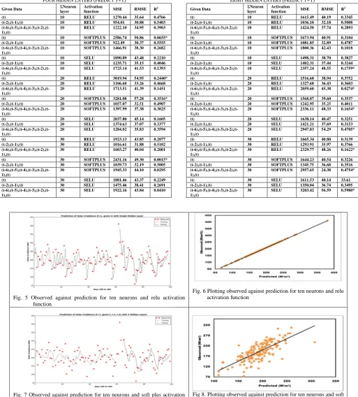
Fig. 5 Observed against prediction for ten neurons and relu activation function
Fig. 6 Plotting observed against prediction for ten neurons and relu activation function
Fig. 7 Observed against prediction for ten neurons and soft plus activation function
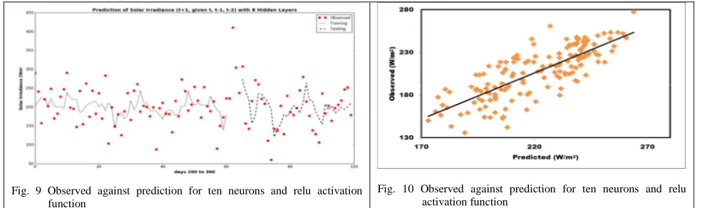
Fig. 9 Observed against prediction for ten neurons and relu activation function
Fig. 10 Observed against prediction for ten neurons and relu activation function
Prediction results of multilayer perceptron can be seen in each view of the figures above with the number of the minimum error. The results are displayed to see the best model for each hidden layer. In Fig. 5 the model generated in a single hidden layer experiment with the best test given data (t) predictive model is present by generating the optimal model; number of neurons = 10, activation function = RELU, MSE = 74.88 W/m2, RMSE = 08.65 W/m2, and R2 = 0.9691, while for distribution of plotting data between observed and prediction seen in Fig. 6.
Data output using this model is more likely forming a straight line on a linear equation. While in Fig. 7, the experiments using four hidden layers with the best test given data (t-2, t-1, t), resulting in an optimal prediction model; number of neurons = 10, activation function = SOFTPLUS, MSE = 922.49 W/m2, RMSE = 30.37 W/m2, and R2 = 0.5555. Plotting data between observed and prediction can be seen in Fig. 8, the distribution of both data using this model has scattered away from the straight line because training and testing data are experimented by adding a hidden layer in its neural network. Fig. 9 shows the experiment using eight hidden layers with optimal data given (t-2, t-1, t) resulting optimal prediction model; number of neurons = 10, activation function = RELU, MSE = 1036.10 W/m2, RMSE = 32.18 W/m2, and R2 = 0.5008, whereas the plotting distribution of data added more away from linear straight line compared to four hidden layers, with increasing hidden layer on the same activation function makes the model performance become worse.
2) Autoregressive Integrated Moving Average (ARIMA)
TABLE IV
PERFORMANCE OF ARIMA MODEL FOR MULTI INPUT SOLAR IRRADIANCE
WITH TUNING MODEL (PREDICT T+1) WITH INPUT (T)
Given Model RMSE MAE MAPE
ARIMA(1, 0, 0) 46.630 36.340 26.115
ARIMA(1, 1, 1) 46.742 35.840 24.254
ARIMA(1, 1, 2) 46.393 35.549 24.569
ARIMA(1, 1, 3) 46.470 35.664 24.621
ARIMA(2, 1, 1) 46.249 35.504 24.600
ARIMA(2, 1, 2) 46.458 35.683 24.626
ARIMA(3, 0, 1) 46.771 36.309 25.956
ARIMA(3, 1, 1) 46.353 35.603 24.624
ARIMA(4, 1, 1) 46.469 35.750 24.649
TABLE V
PERFORMANCE OF THE ARIMA MODEL FOR MULTI-INPUT SOLAR
IRRADIANCE WITH TUNING MODEL (PREDICT T+1) WITH INPUT (T-2,T-1,T)
Given Model RMSE MAE MAPE
ARIMA(1, 1, 2) 45.762 35.272 24.139
ARIMA(1, 1, 3) 45.943 35.598 24.237
ARIMA(1, 1, 4) 45.789 35.56 24.134
ARIMA(2, 1, 1) 45.821 35.488 24.185
ARIMA(3, 0, 1) 46.031 35.738 24.995
ARIMA(3, 0, 2) 46.057 35.752 24.994
ARIMA(3, 1, 1) 45.930 35.490 24.193
ARIMA(4, 1, 1) 45.943 35.682 24.232
ARIMA(4, 1, 2) 45.829 35.366 24.187
TABLE.VI
PERFORMANCE OF ARIMA MODEL FOR MULTI INPUT SOLAR IRRADIANCE
WITH TUNING MODEL (PREDICT T+1) WITH INPUT (T-6,T-5,T-4,T-3,T-2,T-1,T)
Given Model RMSE MAE MAPE
ARIMA(1, 1, 2) 43.914 34.827 23.762
ARIMA(1, 1, 3) 44.222 35.071 23.683
ARIMA(2, 1, 1) 44.054 34.891 23.665
ARIMA(2, 1, 2) 44.150 35.025 23.647
ARIMA(3, 0, 1) 44.115 35.053 24.659
ARIMA(3, 0, 2) 44.186 35.099 24.645
ARIMA(3, 1, 1) 44.186 34.995 23.663
ARIMA(4, 0, 1) 44.138 35.080 24.666
ARIMA(4, 1, 1) 44.065 35.044 23.690
Fig. 11 Observed against prediction for ARIMA(2,1,1) model with given (t) step data
Fig. 12 Plotting observed against prediction for ARIMA(2,1,1) model with given (t) step data
Fig. 13 Observed against prediction for ARIMA(1,1,2) model with given (t-2, t-1, t) step data
Fig. 14 Plotting observed against prediction for ARIMA(1,1,2) model with given (t-2, t-1, t) step data
Fig. 15 Observed against prediction for ARIMA(1,1,2) model with given (t-6, t-5, t-4, t-3, t-2, t-1, t) step data
Fig 16. Plotting observed against prediction for ARIMA(1,1,2) model with given (t-6, t-5, t-4, t-3, t-2, t-1, t) step data
Experimental results of the ARIMA model can be seen in each view of the figure above. The results are shown to present the optimal model for each input data or p,d,q input for created ARIMA model. In Fig. 15, the model generated in ARIMA(1,1,2) with given (t-6, t-5, t-4, t-3, t-2, t-1, t) steps in testing data, can be noted RMSE, MAE, and MAPE gives the most minimum error value among other ARIMA model using generated tuning model. Error values are represented by generating models shown in Table VI. While for the spread of plotting result between observed and prediction can be seen in Fig. 16. Output model represents
of plotting data in Fig. 12 is not better than two previous ARIMA models.
After experimenting on two different models of Multilayer Perceptron and ARIMA, to get the prediction result of each model can be conducted comparing to both. The experimental results compare only to two models that are produced for inputs (t) and (t-2, t-1, t), because two inputs produce optimal predictions and there are slices between the two models. The first model generated by
Multilayer Perceptron with input (t) and single hidden layer compared to ARIMA (2,1,1) with input (t) as shown in Fig. 18. Second is the model generated by Multilayer Perceptron with input (t-2, t-1, t) which has four hidden layers compared to ARIMA(1,1,2) which have the same input as seen in Fig. 17, while the best model obtained in this experiment is Multilayer Perceptron with (t) input and single hidden layer and ARIMA(1,1,2) with (6,5, 4, 3, 2, t-1, t).
Fig 17. Comparison of observed, MLP, and ARIMA data with (t-2,t-1,t) input Fig 18. Comparison of observed, MLP, and ARIMA data with (t) input
III. RESULT AND DISCUSSION
After conducting some experiments using several models of Multilayer Perceptron and ARIMA, several factors need to be observed that influence the output of each model, for Multilayer Perceptron:
1) Transfer function that influences hidden layer: In each table (I-II-III), the RELU function shows consistent performance. This function is non-linear with input x> = 0, mean error result is smaller than the other two activations function. It can be seen the average movement of errors resulting from each layer is almost similar to using this function.
2) Ʃ Neuron layer: The number of neuron layers determines the error value generated by the model. Increasing the value of the neuron/layer and given input data, it will increase the value of MSE and RSME. This will decrease the value of model performance for coefficient determination.
3) Input data: Data input consists of 3 categories to predict t+1. The consecutive input combinations are given t-6 prior seven days, t-2 for prior three days, and t for the main day consist of 1-3-7 consecutive inputs. A single hidden layer with single input t provides an optimal value for each activation function and the hidden layer is used. The best coefficient of determination scores is R2 = 0.9691 with t input to predict t+1. However, at given three data (t-2, t-1, t), the data on each model gives almost the same error value for each hidden layers table. It can also be taken into account as a choice of models whose performance is consistent with the
value of error. In addition, the increasing number of given data, reduce the performance of MSE, RMSE, and R2
4) Hidden layer: Increased hidden layers, then error values on the transfer function and the performance of the model will also decrease. In four hidden layers, the performance of model provided negative (* mark) result if used input (t) data. It seems input (t) data doesn’t create an optimal model for this hidden layer. As well as the input is given in t-6 data not created the optimal model for 8 hidden layers. The optimal model has resulted for a single hidden layer.
of neurons = 10, activation function = RELU, MSE = 1036.10 W/m2, RMSE = 32.18 W/m2, and R2 = 0.5008, whereas the plotting distribution of data added more away from a linear straight line compared to four hidden layers, with increasing hidden layer on the same activation function makes the model performance worse.
While in the ARIMA model experiments, the definition of Autoregressive (p), Moving Average (q), and the parameter of data set (d) are defined. The first model, to get the optimal result conduct tuning model for the combination of p, d, q. input data (t) for the prediction (t+1) obtained combination model is ARIMA(2,1,1), to get the second model of data input (t-2, t-1, t) obtained combination model is ARIMA(1,1,2) and third model with data input (t-6, t-5, t-4, t-3, t-2, t-1, t) obtained combination model is ARIMA(1,1,2). The optimal model obtained RMSE, MAE, MAPE is a model produced by the combination of inputs on the third model. This indicates the predictions of the next seven days produce a small error value compared with the predicted data next one day and the next three days. ARIMA model combination is a linear form of an equation that is performed for time series prediction data.
In both the process of forming model between MLP and ARIMA there are some differences in plotting data. In process of modeling MLP, data distribution in Fig. 6 denser than that of Fig. 8 and 10 since the prediction result is an inconsistency error between observation and prediction data. Numbers of data that has a wide range between observation and precision becomes a contributor to making plotting away from a straight line. The problem occurs due to the increase of hidden layer that makes the model performance decreased. Besides, that large numbers of data will support the formation of models with good learning. The same situation is also found in the ARIMA model. Modeling with the optimal selection of p, d, q through the process of tuning model raises the optimal result. The result of plotting data further widens the range between observation and prediction so that large error contributions make plotting data away from straight lines.
IV. CONCLUSIONS
Predictive model made in this study by using one of the weather parameters of solar irradiance. Time series data is a series of data that have complex problems. In the solution used one of the deep learning models of Artificial Neural Network with the concept of multilayer perceptron and ARIMA with linear regression concept. The experiments of MLP were performed using a hidden layer basis that is divided into three categories; one, four and eight hidden layers. One day prediction (t+1) or single data output with 1-day data input using a multilayer perceptron regression model, while for data input 3-days prior, and 7-days prior using multilayer perceptron window method model. ARIMA model using Autoregressive (p), Moving Average (q), and a parameter of data set (d) to calculated of prediction next data. After experimenting using two models, MLP with Deep Learning approach showed preferable result than using the ARIMA model. MLP model is built to get the smallest possible error value. For performance evaluation use Mean
Squared Error, Root Mean Squared Error and Coefficient of Determination. The results obtained are topology with single hidden layer regression, the number of neurons = 10, activation function = RELU and input data a day prior. This experiment shows the problem time series data not only lies in numbers of data input but the selection of its ANN architecture provides opportunities for many experimental options including determination of weight, activation function and the number of layers. Although ARIMA has model experiment may not optimal predictive results, but MLP has the more minimum error in this experiment. However one should note that the data is compatible with the required model.
REFERENCES
[1] Xinghua Fan, Li Wang, Shasha Li, Predicting chaotic coal prices using a multi-layer perceptron network model, In Resources Policy, Volume 50, 2016, Pages 86-92, ISSN 0301-4207.
[2] Ramón Velo, Paz López, Francisco Maseda, Wind speed estimation using multilayer perceptron, In Energy Conversion and Management, Volume 81, 2014, Pages 1-9, ISSN 0196-8904.
[3] Kumar Abhishek, M.P. Singh, Saswata Ghosh, Abhishek Anand, Weather Forecasting Model using Artificial Neural Network, In Procedia Technology, Volume 4, 2012, Pages 311-318, ISSN 2212-0173.
[4] Kahina Dahmani, Gilles Notton, Cyril Voyant, Rabah Dizene, Marie Laure Nivet, Christophe Paoli, Wani Tamas, Multilayer Perceptron approach for estimating 5-min and hourly horizontal global irradiation from exogenous meteorological data in locations without solar measurements, In Renewable Energy, Volume 90, 2016, Pages 267-282, ISSN 0960-1481.
[5] Ján Vaščák, Rudolf Jakša, Juraj Koščák, Ján Adamčák, Local weather prediction system for a heating plant using cognitive approaches, Computers in Industry, Volume 74, December 2015, Pages 110-118, ISSN 0166-3615.
[6] Seydou Traore, Yufeng Luo, Guy Fipps, Deployment of artificial neural network for short-term forecasting of evapotranspiration using public weather forecast restricted messages, In Agricultural Water Management, Volume 163, 2016, Pages 363-379, ISSN 0378-3774.
[7] Diana A. Bonilla Cardona, Nadia Nedjah, Luiza M. Mourelle, Online phoneme recognition using multi-layer perceptron networks combined with recurrent non-linear autoregressive neural networks with exogenous inputs, Neurocomputing, Volume 265, 2017, Pages 78-90, ISSN 0925-2312.
[8] Mengjiao Qin, Zhihang Li, Zhenhong Du, Red tide time series forecasting by combining ARIMA and deep belief network, Knowledge-Based Systems, Volume 125, 2017, Pages 39-52, ISSN 0950-7051.
[9] Abass Gibrilla, Geophrey Anornu, Dickson Adomako, Trend analysis and ARIMA modelling of recent groundwater levels in the White Volta River basin of Ghana, Groundwater for Sustainable Development, Volume 6, 2018, Pages 150-163, ISSN 2352-801X. [10] Kanika Taneja, Shamshad Ahmad, Kafeel Ahmad, S.D. Attri, Time
series analysis of aerosol optical depth over New Delhi using Box– Jenkins ARIMA modeling approach, Atmospheric Pollution Research, Volume 7, Issue 4, 2016, Pages 585-596, ISSN 1309-1042. [11] S. Chattopadhyay, G. Chattopadhyay, Univariate modelling of summer-monsoon rainfall time series: comparison between ARIMA and ARNN, CR Geoscience, 342 (2010), pp. 100-107.
[12] George E. P. Box, Gwilym M. Jenkins, Gregory C. Reinsel, Greta M. Ljung, Time Series Analysis: Forecasting and Control, 5th Edition, ISBN: 978-1-118-67502-1, Jun 2015.
[13] Parag Sen, Mousumi Roy, Parimal Pal, Application of ARIMA for forecasting energy consumption and GHG emission: A case study of an Indian pig iron manufacturing organization, Energy, Volume 116, Part 1, 2016, Pages 1031-1038, ISSN 0360-5442.