Hybrid Preprocessing Method for Support Vector Machine for Classification of Imbalanced Cerebral Infarction Datasets

Vol.9 (2019) No. 2

ISSN: 2088-5334

Hybrid Preprocessing Method for Support Vector Machine for

Classification of Imbalanced Cerebral Infarction Datasets

Zuherman Rustam

#1

, Dea A. Utami

#

, Rahmat Hidayat

*

, Jacub Pandelaki

+

, Widyo A. Nugroho

+

,#

Department of Mathematics, University of Indonesia, 16424 Depok, Indonesia E-mail: [email protected]

*

Department of Information Technology, Politeknik Negeri Padang, Padang, Sumatra Barat, Indonesia

+

Department of Radiology, Cipto Mangunkusumo Hospital, Jakarta 10430, Indonesia

Abstract— Cerebral infarction is one of the causes of ischemic stroke in the brain, and machine learning can be used in the detection

of cerebral infarction in the brain. In diagnosing the presence of cerebral infarction in the brain, machine learning is used because it is not enough just to use a CT scan to diagnose. Support vector machine (SVM) is a machine learning method that is known for its high accuracy value. However, SVM can produce less optimal results if the data used is imbalanced. If imbalanced data is used, the resulting model will be biased. Therefore, this study uses a hybrid preprocessing method for SVM on the classification of an imbalanced cerebral infarction dataset obtained from the Department of Radiology at Dr. Cipto Mangunkusumo Hospital. This method is a combination of several sampling methods that deal with the problem of imbalanced data and utilizes undersampling and oversampling techniques in combination with SVM. Oversampling modifying the infarction dataset through the duplication of data with a small number of classes to be balanced with a large number of data classes. While undersampling reducing data with a large number of classes to be balanced with a smaller number of data classes. Undersampling and Oversampling are combined into a hybrid method. This method is a hybrid method of the undersampling and oversampling that can be used in SVM. The results of hybrid method using SVM will be compared with the undersampling and oversampling using SVM, individually. And SVM method without preprocessing the imbalanced dataset. The accuracy of the proposed method reached 94% in our evaluations for SVM using a hybrid preprocessing method.

Keywords— hybrid preprocessing method; support vector machine; undersampling; oversampling; imbalanced Data; classification of

cerebral infarction; ischemic stroke.

I. INTRODUCTION

In Indonesia, stroke is the third deadliest disease, exceeded only by heart disease and cancer. From the data at Southeast Asia Medical Information Center, it is known that the highest mortality rate resulting from stroke occurs in Indonesia, followed by the Philippines, Singapore, Brunei, Malaysia, and Thailand. Ischemic stroke is the most common type of stroke in Indonesia, accounting for 52.9% of all stroke patients.

Stroke is a disease that occurs due to circulatory disorders, which are caused by the presence of blockages (infarction) or ruptured blood vessels in the brain [1]. This infarction of blood vessels in the brain can be caused by the presence of blood clots in the heart or in other blood vessels [1]. When a stroke occurs, tissue in the brain will die, which can stop the circulation of blood carrying oxygen and nutrients to the body [2].

In general, strokes are classified into two types, as hemorrhagic stroke or ischemic stroke. Hemorrhagic stroke is caused by an increase in acute blood pressure, or by other diseases that cause weak blood vessels [3]. Meanwhile, ischemic stroke is caused by a blockage of the arteries due to emboli, or by atherosclerosis in the blood vessels of the brain [3]. Blockage of the arteries is called infarction. In ischemic stroke, cerebral infarction is the more common condition, and is the death of brain cells due to prolonged ischemia [3].

For patients with ischemic stroke, a cerebral infarction can bee seen in the brain through detection with a CT scan. However, the results of a CT scan are not enough to detect and diagnose the presence of infarction in the brain. Machine learning can be used to assist in the detection and classification of infarcts in the brain using labels and features available from the results of CT scans.

classification method to classify datasets of cerebral infarction in the brain leading to ischemic stroke. A dataset was obtained from the Department of Radiology at Dr. Cipto Mangunkusumo Hospital (RSCM). However, because infarction data is not balanced, the imbalanced tendency of the class data will cause instability, and the data will be more inclined to classification as classes composed of larger numbers.

The problem of imbalanced data is solved by modifying the infarction dataset through the duplication of minority data, or data with a small number of classes, to be balanced with data with a large number of data classes [4]. This process is also called oversampling. Other datasets are modified by reducing majority data, or reducing data with a large number of classes, to be balanced with a smaller number of data classes [4]. This process is also called undersampling.

There are several studies that have discussed this resampling technique, including Burez et al [5], who investigated the impact of CUBE random undersampling and other sophisticated undersampling techniques on imbalanced datasets to predict customers churn. The modeling techniques used were random weighting, increasing gradient, logistic regression, and random forest. The results of the study show that the technique has not been very successful.

Amin et al [6] presented research on retrieval techniques for rulemaking in unbalanced datasets to include the SMOTE and MWMOTE techniques using genetic algorithms. Vafeiadis et al [7] presented a comparative study of Neural Network algorithms, SVM, Decision Tree, Naïve Bayes and Logistic Regression for churn prediction systems. Based on the results of their study, SVM was shown to be the algorithm that produces the best accuracy among other algorithms.

This study uses a hybrid preprocessing method that combines oversampling and undersampling methods to achieve results that are more accurate. After preprocessing on imbalanced data, balanced data is used as input for SVM classifiers that classify the presence of cerebral infarction that can lead to ischemic stroke. Our primary motivation is to determine how the hybrid preprocessing method influences the prediction accuracy of infarction data by calculating the model accuracy using SVM classifiers.

II. MATERIAL AND METHODS

A. Oversampling

Oversampling is a technique for the process of resampling with imbalanced data. Minority class data samples are duplicated to balance them with data that have larger numbers of data classes [8]. Mathematically, the oversampling method can be explained through the below equation [9] :

| ′ | ← |

| ∪ | |

(1)

Where S is training data and E is synthetic data. Various oversampling techniques are used in duplicating the data to appropriately improve the performance of algorithms. In this study, the oversampling technique used is the Synthetic Minority Oversampling Technique.

B. Synthetic Minority Oversampling Technique (SMOTE)

The Synthetic Minority Oversampling Technique (SMOTE) [10] is an oversampling technique that adds new synthetic data to minority classes to balance them with the majority class sample. The parameters used are the percentage of minority classes that are exceeded, the total number of minority class data, and data parameters that state the value of the nearest neighbor of the minority class to the majority class. First, the algorithm finds the value of k, which is the value of the nearest neighbor to each sample of the minority class using a measure of Euclidean distance [11]. Synthetic data is generated along with line segments that are joined by samples of the original minority classes with the k of their closest neighbors [11]. The value of k depends on the amount of synthetic data needed [11].

Steps in sampling synthesis [12]:

• Generate a random number between 0 and 1

• Calculate the difference between feature vectors of minority class samples to their closest neighbors

• The result of calculating the difference between the vectors will be doubled with the random number generated in step number 1

• Add the multiplication results from Step 3 to the minority class feature vector

• Identify the newly created sample with the resulting feature vector.

C. Undersampling

Undersampling is also a technique for the process of resampling with imbalanced data. A portion of the majority class sample is removed to balance it with the minority sample [10]. Mathematically, the undersampling method can be explained through the below equation [9] :

|

〖

^′

〗

_max | ← | _max | ∩ | |

(2)

Where S is training data and E is syntheticdata. A number of measured observations for | |are taken randomly from the majority class , resulting in a majority class with the new size ′

| | ← |

| ∪ |

|

(3)

Then a new data ′ is formed by combining the observations of the minority class and the new majority class ′

| | ← |

| ∪ |

| ∩ | |

(4)

D. Edited Nearest Neighbor (ENN)

used in research. In this study, the method used is a hybrid preprocessing method based on SMOTE, Edited Nearest Neighbor, and SVM.

E. Hybrid Preprocessing Method

This method is a combination of SMOTE and ENN methods for oversampling and undersampling, respectively, and is used to balance the dataset. Some majority class samples that are deleted are added to the minority class sample [11], to enhance performance relative to the performance of the techniques when used individually. The hybrid method used in this study is SMOTEENN (SMOTE+ENN), which applies rules to data cleansing by deleting several data samples from both classes [11]. Samples of data to be deleted are selected based on the number of closest neighbors that are misclassified [11]. That is, if the closest neighbors from any sample data are misclassified, they are removed from the training data.

F. Support Vector Machine (SVM)

SVM is a machine learning technique that includes supervised learning. SVM aims to minimize structural risk and account for aspects of generalization by finding the best hyper plane to separate data from defined classes [14]. The best hyper plane has the largest margin with the smallest error [15], where margin is the distance between the first class hyper plane and the second-class hyper plane [15]. The class hyper plane is comprised the class data points closest to the hyper plane, which are called support vectors [15].

Suppose there is a data , , ! where " = 1,2, … . , and

! ( − 1,1 with ! are class labels of the infarct dataset,

namely infarct class and normal class. The hyper plane that will be formed is defined by the following equation:

!( ) = *

+

_{+ -}

₍₅₎

where . is a vector of the weight parameter values, and b is a bias that has a scalar value. The formed hyperplane will separate the data into two classes on the infarction dataset, namely the infarct class and the normal class, or the class SVM method that has positive and negative values. The process of separating these datasets is carried out with the following conditions:

.

+

_{+ - ≥ 1, ! = +1}

₍₆₎

.

+

_{+ - ≤ 1, ! = −1}

₍₇₎

The above equations in general can be stated in the following statement:

! (.

+

_{+ -) ≥ 1 , " = 1,2, … , 1}

₍₈₎

The distance between the two hyperplanes can be defined with the equation below:

2.3 4562

‖.‖

=

‖.‖8 (9)

The resulting total distance between the two hyper planes is 9

‖.‖. To maximize margins, ‖w‖ is minimized by

min

8₉

‖.‖

9

₍₁₀₎

If training data is not linearly separated, then a slack < variable can be added which is used as a misclassification of the noisy example. Adding slack variables changes the formula to the following:

min

8₉

‖*‖

9

_{+ = ∑ <}

₍₁₁₎

with the provision of

! (.

+

_{+ -) ≥ 1 − <}

₍₁₂₎

and

< ≥ 0 ∀" = 1,2, … , 1

(13)

If < > 1, there will be misclassification at that point.

There is a parameter C that is used to avoid overfitting, and it is referred to as the soft margin classification.

To produce the optimal solution, the Lagrange duality theorem is used, and the formula below is a decision function of SVM :

B( ) = CB1(∑_(" = 1)^D▒

〖

!_" F_" G( _", ) +

H^ ∗

〗

) C. J. 0 ≤ F_" ≤ =

(14)

where Fis the Lagrange duality solved by the quadratic optimization problem, H∗shows the optimum bias value, and

G( , ) is the kernel function which is expressed as:

GK ,

L

M = N O P−

Q 4R SQ

T

UT

V

(15)

where, the kernel function used in this study is the kernel Radial Basis Function (RBF).

G. Kernel Function

The kernel function resolves problems that are linear in order to be applied to non-linear problems [14]. Especially for algorithms expressed in inner product between two vectors [14]. In this study, kernel functions are used in Support Vector Machine. In finding support vectors, it takes the dot product results from a data that has been transformed into a new space that has a higher dimension [15]. The transformation

∅

is usually hard to know, so it can be replaced by the kernel function G( , _L), which can be defined as transformation

∅

implicitly [15]. Therefore, the equation of the kernel trick is as follows:

GK ,

L

M = ∅( ). ∅K

L

M

(16)

X

9

_{Y∅( ), 〖∅( 〗}

L

M\ = Q∅( ) − 〖∅( 〗

L

MQ

9

=

2 Y1 − GK ,

L

M\

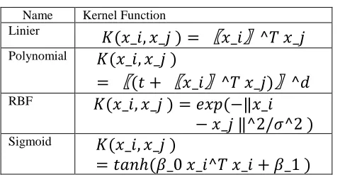
(17)

There are several kernel functions with the parameters in table I

TABLEI

THE SEVERAL KERNEL FUNCTION

Name Kernel Function Linier

_{G( _", _] ) =}

〖

_"

〗

^^ _]

Polynomial

G( _", _] )

=

〖

(J +

〖

_"

〗

^^ _])

〗

^X

RBF

G( _", _] ) = N O(−‖ _"

− _] ‖^2/F^2 )

Sigmoid

G( _", _] )

= JH1ℎ(a_0 _"^^ _" + a_1 )

In this study, the kernel function used is the kernel Radial Basis Function (RBF). The RBF kernel is often used with SVM classification. From the above equation, there is

Q − LQ9 which is called the Euclidean square distance,

which is the distance between two feature vectors. σ _{is a free}

parameter that is not zero [14], [15].

H. proposed method

First, a classification model is built for infarction data. The dataset used consists of 70% training data and 30% testing data. A Python program is used to determine the presentation of sample accuracy for the minority data class and the majority data class, where the minority data class is a positive data class (i.e., there is infarction in the brain) and the majority data class is a negative data class (i.e., there is no infarction in the brain). The number of samples of the minority and majority class data is denoted by b and

b respectively.

Second, resampling techniques are used to balance the training data samples [4]. Either data samples from minority classes are added with synthetic data obtained using oversampling techniques, or data samples from the majority class are omitted based on the value of the nearest neighbor k from the data obtained using undersampling techniques [4]. The oversampling and undersampling techniques are then combined into a hybrid resampling method to achieve good classification performance.

Third, the data classification model is trained using the SVM classification. In this stage, some data training will be conducted. Among them is training data before and after using resampling techniques with SVM classification. After that, predictions are made on the data and will be compared with the results of the prediction mentioned above.

III.RESULT AND DISCUSSION

A. Data

The data used in this study are from ischemic stroke patients who have cerebral infarction in their brain. Data was

taken from January to November 2018 from Dr. Cipto Mangunkusumo Hospital. This infarction data amounted to 156 data with 7 features proportioned as 70% training data and 30% testing data from the original data, with actual amounts of 103 major data and 53 minor data. Minor data represent data classes that indicate the presence of infarction, and the label ‘1’ is used for the dataset, while the major data represent data classes that do not indicate infarction, and the label '0' is used for the dataset. Table II explains the infarction data features that will be examined.

TABLEII

THE FEATURES OF CEREBRAL INFARCTION DATASET

No Feature Definition of feature

1 Area The size of the area from the infarction point

2 Min The minimum value of infarction

3 Max The maximum value of infarction

4 Average The average value of infarction

5 SD Standard error value of infarction

6 Sum The sum value of infarction point

7 Length Length of infarction point

B. Metric Evaluation

Metric evaluation of this method is needed to determine that the method proposed in this study can solve the classification problem of the presence of cerebral infarction in the brain leading to stroke. An evaluation was carried out based on the values of Accuracy, Recall, Precision, and f-score.

TABLEIII CONFUSION MATRIX

Predicted Class

Positive Class Negative Class

Actual Class

Positive Class TP FN

Negative Class FP TN

Information :

TP: True Positive: Infarction is predicted, and infarction is present FP: False Positive: Infarction is predicted, and infarction is not present

FN: False Negative: Absence of infarction is predicted, and infarction is present

TN: True Negative: Absence of infarction is predicted, and no infarction is present

Confusion matrices for the SVM method alone, the SVM method with SMOTE, SVM method with ENN, and the SVM method with the Hybrid Method (SMOTEENN) are shown in Table IV, Table V, Table VI and Table VII respectively.

TABLEIV

CONFUSION MATRIX FOR THE SVM METHOD WITHOUT RESAMPLING

Predicted Class

Positive Class Negative Class

Actual Class

Positive Class 27 4

TABLEV

CONFUSION MATRIX FOR THE SVM METHOD WITH SMOTE

Predicted Class

Positive Class Negative Class

Actual Class

Positive Class 28 3

Negative Class 1 15

TABLEVI

CONFUSION MATRIX FOR THE SVM METHOD WITH ENN

Predicted Class

Positive Class Negative Class

Actual Class

Positive Class 30 2

Negative Class 3 12

TABLEVII

CONFUSION MATRIX FOR THE SVM METHOD WITH THE HYBRID METHOD

(SMOTTENN)

Predicted Class

Positive Class Negative Class

Actual Class

Positive Class 32 2

Negative Class 1 12

1) Accuracy of classification: The classification accuracy is the average number of samples categorized or predicted correctly by the classifier. The greater the value for Accuracy of classification, the better the performance of the method.

cddeDHd! fg =hHCC"g"dHJ"f1 =_{(ki5+j5kj5+i)}(+i5+j) (18)

2) Recall or True Positive Rate: Recall is the coverage

of a model in predicting a particular class. The greater the value of Recall, the better the performance of the method.

lNdHhh =

_(ki5+j)+j (19)

3) Specificity or True Negative Rate: Specificity is the

prediction of the negative class sample test with the overall negative class sample. The higher the value of the Specificity, the better the performance of the method.

ONd"g"d"J! =

_(kj5+i)+i (20)

4) Precision or Positive Predictive Value: Precision is

the ratio of the test positive sample class that is predicted correctly with the overall positive class sample. The higher the value of Precision, the better the performance of the method.

mDNd"C"f1 =

_(kj5+j)+j (21)

5) f-score: The f-score is the average harmonic

between Precision and Recall. The best classifiers have a value close to 1 and the worst classifiers have a value close to 0.

g1 = 2 × Y

jopq r s × tpq uu_{jopq r s 5tpq uu}

\

(22)

C. Result

Table VIII shows the results of the accuracy of the entire method used, both before and after resampling techniques with SVM classification.

TABLEVIII

ACCURACY OF EACH METHOD

Accuracy Data Training Data Testing

SVM 87% 70% 30%

SVM with ENN 89% 70% 30%

SVM with SMOTE 91% 70% 30%

SVM with

SMOTEENN 94% 70% 30%

As listed in table VIII, the best accuracy obtained was 94%, which resulted from the SVM classification method using data that was sampled with SMOTEENN. Meanwhile, the lowest level of accuracy resulted from the SVM classifiers using data without the use of a resampling technique and was equal to 87%. Table IX shows the overall performance of the SVM classification model, both before and after the use of resampling techniques on the infarction data.

TABLEIX

CLASSIFICATION REPORT FOR EACH METHOD

As listed in Table IX, the SVM with SMOTEENN method had better performance than the other methods used, with a recall value of 91%. This was followed by the SVM with ENN method with a recall value of 89%. Based on the precision values obtained, the SVM with SMOTEENN and SVM with ENN methods demonstrated the best results, with values of 92%. However, based on the specificity value, the SVM with ENN method demonstrated better results than the SVM with SMOTEENN method as well as other methods, with a value of 96%. Because all methods in this study have f-score close to 1, they are all good methods for classification of the presence of infarction in the brain leading to stroke. However, highest f-score resulted from the SMOTEENN method, with a value of 91%. Based on the f-score, the best method is the SMOTEENN method.

Table X shows the overall performance of the SVM classification model in the class 0 data sample (negative class that does not have brain infarction) both before and after resampling techniques. The data sample class 0 is the majority data sample.

Accuracy Precision Recall Specificity f-score

SVM 87% 87% 87% - 87%

SVM

with ENN 89% 92% 89% 96% 90%

SVM with SMOTE

91% 88% 88% 88% 88%

SVM with SMOTEE

NN

TABLEX

CLASSIFICATION REPORT FOR EACH METHOD IN MAJORITY CLASS

Based on the recall values listed in Table X, the SVM with SMOTEENN method is better relative to other methods, with a recall value of 94%, followed by the SVM method without using resampling techniques, with a recall value of 90%. Based on the precision values, the SVM with ENN method is the best method for handling problems of the majority class, with precision values of 100%, followed by the SVM with SMOTEENN method, with precision values of 94%. The SVM with ENN method is also the best method based on the specificity values, with a value of 100%. Because all the methods in this study have f-score close to 1, they are all good methods for sampling this majority class data. However, the highest f-score resulted from the SMOTEENN method, with a value of 94%. Based on the f-score, the best method is the SMOTEENN method.

Table XI shows the overall performance of the SVM classification model in the class 1 data sample (positive class of infarction in the brain) both before and after the resampling technique was performed. Class 1 data samples are minority data samples.

TABLEXI

CLASSIFICATION REPORT FOR EACH METHOD IN MINORITY CLASS

A

cc

u

ra

cy Precision Recall Specificity

f-score

SVM 87% 85% 73% - 79%

SVM with

ENN 89% 71% 100% 86% 83%

SVM with

SMOTE 91% 79% 88% 87% 83%

SVM with

SMOTEENN 94% 88% 88% 94% 88%

Based on the recall values in the Table XI and figure 4, the SVM with ENN method is the best relative to other methods, with a recall value of 100%, followed by the SVM with SMOTE methods and SVM with SMOTEENN methods with recall values of 88%. Based on the precision values, the SVM with SMOTEENN method is the best method, with a precision value of 88%, followed by the SVM method without a resampling technique, with a precision value of 85%. The SVM with SMOTEENN method is also the best method based on the specificity values, with a value of 94%, followed by the SVM with

SMOTE method, which is good at handling this minority class problem, with a specificity value of 87%. Based on the f-score, the SVM with SMOTEENN method is the best method, with an f-score of 88%.

In this study, we examined an imbalanced data class sample from a hospital-regarding cerebral infarction. The data had 103 majority data and 53 minority data. Evaluations were carried out for resampling techniques including the ENN Undersampling technique, the SMOTE Oversampling technique, and the SMOTEENN hybrid resampling technique, which combines the SMOTE and ENN techniques. After resampling the data, the balanced data was tested using SVM classifiers to predict the classification of cerebral infarction in the brain leading to ischemic stroke. The main objective of this study was to improve the classification performance of machine learning algorithms for the prediction of minority and majority classes. We compared SVM classifiers without the use of resampling techniques in training data against SVM classifiers using resampling techniques on training data, for both minority and majority classes. This method produces increased performance for SVM because of the imbalanced data class samples being deleted based on the number of closest neighbors, preventing misclassification in the data. The hybrid method achieved the highest accuracy, at 94%.

IV.CONCLUSION

Predicting the presence of cerebral infarction in the brain of a patient assists hospital radiologists in diagnosing ischemic stroke in patients, as one of the causes of ischemic stroke is cerebral infarction, or the blockage and rupture of blood vessels in the brain.

The experimental results show that the performance of SVM classifiers is improved by the use of resampling techniques to rebalance the infarct data, which allows. SVM to properly and correctly predict the data. Based on our results, the SVM with SMOTEENN method provides the best classification of cerebral infarction. This method is a hybrid of SVM with ENN and SVM with SMOTE and it can produce better accuracy relative to that of their use individually.

ACKNOWLEDGMENTS

The Indonesian Ministry of Research and Higher Education financially supported this research, with a PDUPT 2018 research grant scheme (ID number 389/UN2.R3.1/HKP05.00/2018). We thank all reviewers for the improvement of this article.

REFERENCES

[1] V.Bay, B.F.Kjolby, N.K.Iversen et al., “Stroke Infarct Volume Estimation in Fixed Tissue : Comparison of Diffusion Kurtosis Imaging to Diffusion Weighted Imaging and Histology in a Rodent MCAO Model”, PLoS ONE, vol. 13, no.4, e0196161, 2018. [2] G.Wang, J.Jing, Y.Pan, et al., “Does All Single Infarction have

Lower Risk of Stroke Reccurence Than Multiple Infarctions in Minor Stroke?”, BMC Neurology, vol. 19, no.7, 2019.

[3] I.A.Mentari, R.Naufalina, M.Rahmadi, J.Khotib, “Development of Ischemic Stroke Model By Right Unilateral Common Carotid Artery Occlusion (RUCCAO) Method”, Fol Med Indones, vol.54, no.3, pp.200-206, 2018.

Accuracy Precision Recall Specificity _score f-

SVM 87% 88% 90% - 91%

SVM with

ENN 89% 100% 86% 100% 92%

SVM with

SMOTE 91% 93% 87% 88% 90%

SVM with

[4] M.F.Kabir, S.A.Ludwing, “Classification of Breast Cancer Risk Factors Using Several Resampling Approaches”, 17th IEEE International Conference on Machine Learning and Applications, 2018.

[5] J.Burez, D.Van den Poel, “Handling Class Imbalanced in Customer Churn Prediction”, Expert Systems with Applications, vol.36, no.3, pp.4626-4636, 2009.

[6] A. Amin, S. Anwar, A. Adnan et al., “Comparing oversampling techniques to handle the class imbalance problem: A customer churn prediction case study”, IEEE Access, vol. 4, pp. 7940-7957, 2016. [7] T.Vafeiadis, K.I.Diamantaras, G. Sarigiannidis, K.C.Chatzisavvas,

“A Comparison of Machine Learning Techniques for Customer Churn Prediction”, Simulation Modelling Practice and Theory, vol.55, pp.1-9, 2015.

[8] M.Buda, A.Maki, M.A.Mazurowski, “A Systematic Study of The Class Imbalance Problem in Convolutional Neural Network”, Neural Network, vol. 106, pp. 249-259, 2018.

[9] H.He, E.A.Garcia, “Learning from Imbalanced Data”, IEEE Transactions on Knowledge and Data Engineering, Vol.21, No.9, 2009.

[10] D.S.Sisodia, U.Verma, “The Impact of Data Re-Sampling on Learning Performance of Class Imbalanced Bankruptcy Prediction

Models”, International Journal on Electrical Engineering and Informatics, vol.10, no. 2, 2018.

[11] J.Luengo, A. Fernandez, S.Garcia, F.Herrera, “Addresing Data Complexity for Imbalanced Data Sets :Analysis of SMOTE-based Oversampling and Evolutionary Undersampling”, Soft Comput, vol. 15, pp.1909-1936, 2018.

[12] U.R.Salunkhe, S.N.Mali, “Hybrid Approach for Class Imbalance Problem in Customer Churn Prediction : A Novel Extension to Under-Sampling”, I.J.Intelligent Systems and Applications, vol.5, pp.71-81, 2018.

[13] H.Guo, X.Diao, H.Liu, “Embedding Undersampling Rotation Forest for Imbalanced Problem”, Hindawi Computational Intelligence and Neuroscience, 2018.

[14] J.Liu, E.Zio, “Integration of Feature Vector Selection and Support Vector Machine for Classification of Imbalanced Data”, Applied Soft Computing Journal vol.75, pp. 702-711, 2017.