COMPONENT MODE SYNTHESIS AND CHAOS POLYNOMIAL EXPANSION FOR DYNAMIC ANALYSIS OF NON LINEAR LARGE STRUCTURE WITH UNCERTAIN PARAMETERS

34

COMPONENT MODE SYNTHESIS AND CHAOS

POLYNOMIAL EXPANSION FOR DYNAMIC ANALYSIS

OF NON LINEAR LARGE STRUCTURE WITH

UNCERTAIN PARAMETERS

*Mohammed Lamrhari, **Driss Sarsri,***Lahcen Azrar, *Miloud Rahmoune, *Khalid Sbai *Laboratoire d’Etude des Matériaux Avancés et Applications,

FS–EST, University Moulay Ismail, Meknes, Morocco ** Laboratoire des Technologies Innovantes ENSA, University Abdelmalek Essaadi, Tanger, Morocco

*** Equipe Modélisation Mathématique et Contrôle FST, University Abdelmalek Essaadi, Tanger, Morocco

ABSTRACT

The aim of this work is to estimate the non-linear stochastic dynamic response for a reasonable calculation cost. For that, we propose an original approach based on the coupling of the Polynomial Chaos Expansion PCE with Component Mode Synthesis CMS condensation method. CMS method proved to be effective in reducing the size of the problem, while the PCE method allows taking problems with uncertain parameters. This approach allows a minimal computational cost. Otherwise, we present some numerical simulations demonstrate the effectiveness and applicability of the proposed approach.

Keywords: Component Mode Synthesis, non-linear stochastic dynamic response, Polynomial Chaos Expansion, uncertain parameters.

INTRODUCTION

Nonlinear phenomena in the dynamics of structures are relatively well known and many methods have been developed to take these into account when dimensioning a structure. Nevertheless, most of these methods are deterministic and do not allow us to consider the uncertainties present in such structures. Indeed, due to the manufacturing process, there is dispersion on the values of physics parameters, so the latter can be considered as random. Also for a robust design objective, it is necessary to integrate these variations to estimate the associated nonlinear random response.

Furthermore, another form of development is a Polynomial Chaos Expansion (PCE) [5,6]. The stochastic solution may be expanded in terms of the polynomial chaos basis whose elements are obtained from orthogonal polynomial [7]. The properties of this polynomial basis are used to generate a system of deterministic equations. The resolution of this system is used to determine the variability of the response.

However, nonlinear dynamics, the large number of degrees of freedom due to the mesh of a large structure and higher order developing for modeling uncertainty induced a considerable increase of deterministic equations.

One way to solve this problem is the reduction by Component Mode Synthesis (CMS) method proposed in the literature [8-15]. This method allows condensing the large number of degrees of freedom in a small number using the generalized coordinates. Adrian Fritz et al [16] proposed a comparative study of different bases for reduction in nonlinear dynamics structures. Thus, in the CMS method, the overall structure is divided into sub-structures, each of which is analyzed independently in order to obtain the corresponding solution. These solutions are combined to obtain the overall solution of the structure by imposing constraints on the interfaces. The different methods are classified according to CMS interface: fixed interface [8] free interface [9-10], or hybrid interface [11,12].

Recently Sarsri et al [17-18] developed an approach coupling CMS reduction method and developing uncertainty by a polynomial chaos expansion to calculate the frequency transfer functions and response temporal for linear stochastic structures. Sinou J. et al [19] proposed for simple structures, requiring no reduction, a technique taking into account uncertainties in nonlinear models, by combining the method of Harmonic Balance Method (HBM) and developing uncertainty by a polynomial chaos expansion. This method is based on a formulation of nonlinear dynamic problem in which the physical parameters, nonlinear forces and the excitation force are considered random.

The aim of this work is to estimate the stochastic nonlinear dynamic response for a large structure with a minimal computational cost. To do this, we develop a methodological approach for calculating the temporal response of large structures with uncertain parameters. This approach is based on coupling of the Polynomial Chaos expansion with the reduced method (CMS). First, we develop the nonlinear dynamic equations considering geometrical nonlinearities. The resolution of the nonlinear dynamics problem by the Finite Element FE method is adopted. Then, the temporal integration by Newmark is developed. Secondly, we take the random phenomena using the PCE method. The method of stochastic finite element is used. Various types of CMS interface method is used to optimally reduce the model size. The first moments of the nonlinear dynamic response of the reduced system are compared with the entire system. Several numerical simulations have shown the accuracy and efficiency of procedures and methodologies developed

REDUCTION BY COMPONENT MODE SYNTHESIS METHOD

36

taking into account the interface couplings between the sub-structures, after the reduced system is solved. Finally the complete system solution is reconstituted.

The finite element model of the entire structure is partitioned into N substructures SS(i) (i=1,…, N). The equations of motion for each non- linear substructures SS(i) are:

𝑀 𝑖 _𝑢 𝑖 _{+ 𝐶} 𝑖 _𝑢 𝑖_{+ 𝐾} 𝑖 _𝑢 𝑖_{+ 𝐹}

𝑛𝑙 𝑖 = 𝐹𝑒 𝑖 (1)

With 𝑀 𝑖_{, 𝐶} 𝑖 _{and 𝐾} 𝑖 _{are respectively the mass matrix, the damping matrix and the stiffness}

matrix for substructures SS(i).

The displacement vector u i _{is partitioned into a vector u} j

i

, called interface DOF and uin i is

the vector of internal DOF:

u i= _uuj

in i

(2)

The external force vector Fe i is composed into vectors Fej i

and Fee i, called interface force

and external applied force.

𝐹𝑒 𝑖 = 𝐹𝑒𝑗 𝑖

+ 𝐹_𝑒𝑒 𝑖 ₍₃₎

The non linear force vector Fnl iis composed into vectors Fnlj i

and Fnle i, called interface force

and external non linear force.

𝐹𝑛𝑙 𝑖 = 𝐹𝑛𝑙𝑗 𝑖

+ 𝐹_𝑛𝑙𝑒 𝑖 ₍₄₎

In the component mode synthesis methods, the physical displacements of the substructure SS(i) are expressed as a linear combination of the substructure modes. After some algebraic transformations, a set of Ritz vectors Q is obtained and the displacement vector of each sub-structure can be expressed as:

𝑢 𝑖 = 𝑄 𝑖 𝑢𝑗

𝑖

𝜂_𝑝 𝑖 = 𝑄

𝑖 _𝑢

𝑐 𝑖 (5)

With η_p i are the generalized coordinates. The matrix Q i is defined according to the method of sub structuring used (fixed or free interface [10]).

The conservation of interface DOF allows assembling these matrices as in the ordinary finite element methods. Let us denote by uc the vector of independent displacements of the assembled

structure:

𝑢𝑐 =

𝜂𝑝 1

⋮ 𝜂_𝑝 𝑁

𝑢_𝑗

(6)

each substructure SS(i) the following relation:

𝑢𝑐 𝑖 = 𝛽 𝑖 𝑢𝑐 (7)

Where β i is the matrix of localization or of geometrical connectivity of the SS(i) substructure. It makes possible to locate the DOF of each substructure SS(i) in the global DOF of the assembled structure. They are the Boolean matrices whose elements are 0 or 1.

A transformation matrix can be defined for each substructure SS(i) by:

𝑍 𝑖 _{= 𝑄} 𝑖 _𝛽 𝑖 ₍₈₎

Where Q i _{is given by the considered CMS method.}

The displacement vector u i are then given by

𝑢 𝑖 _{= 𝑍} 𝑖 _𝑢

𝑐 (9)

Inserting Eq. (9) into Eq. (1) and multiply on the right by t Z i, using the sum for all substructures, the following equation is obtained:

𝑀_𝑐 𝑢 _𝑐 + 𝐶_𝑐 𝑢 _𝑐 + 𝐾_𝑐 𝑢_𝑐 + 𝑁 𝑡 𝑍 𝑖

𝑖=1 𝐹𝑛𝑙𝑗

𝑖

+ 𝐹_𝑛𝑙𝑒 𝑖 ₌ 𝑡 _𝑍 𝑖_{( 𝐹} 𝑒𝑗

𝑖 𝑁

𝑖=1 + 𝐹𝑒𝑒 𝑖)

(10)

Where: 𝑀𝑐 = 𝑁𝑖=1 𝑡 𝑍 𝑖 𝑀 𝑖 𝑍 𝑖

𝐶𝑐 = 𝑁𝑖=1 𝑡 𝑍 𝑖 𝐶 𝑖 𝑍 𝑖 (11)

𝐾𝑐 = 𝑁𝑖=1 𝑡 𝑍 𝑖 𝐾 𝑖 𝑍 𝑖

Using the interface DOF compatibility of displacements, it can easily be shown that: 𝑡 𝑍 𝑖 _𝐹

𝑒𝑗 𝑖

= 0

𝑁

𝑖=1 (12)

Finally, the reduced equation of motion can be written as follows:

𝑴𝒄 𝒖 𝒄 + 𝑪𝒄 𝒖 𝒄 + 𝑲𝒄 𝒖𝒄 + 𝑵𝒊=𝟏 𝒕 𝒁 𝒊 𝑭𝒏𝒍𝒋 𝒊

+ 𝑭_𝒏𝒍𝒆 𝒊 ₌ 𝒕 _𝒁 𝒊 _𝑭 𝒆𝒆 𝒊 𝑵

𝒊=𝟏

(13)

POLYNOMIAL CHAOS EXPANSION METHOD

In this section, the Polynomial Chaos Expansion and the CMS approaches, presented in the previous sections, will be coupled in order to analyze the dynamic behaviours of structures with uncertain parameters. Based on the CMS, the reduced random differential system to be solved is equation (13)

In the following, the physical properties of each substructure SS(i) described by the mass, damping and stiffness matrices are assumed to be uncertain. 𝑀 𝑖_{, 𝐶} 𝑖 _{and 𝐾} 𝑖 _{are random matrices. The}

38

Using a particular formulation of the stochastic finite element method the matrices 𝑀 , 𝐶

and 𝐾 can be represented in the form:

𝐾 𝑖 _{= 𝐾} 𝑘 𝑖 𝐾

𝑘=0 . 𝜉𝑘 𝐶 𝑖 = 𝐶𝑐=0 𝐶𝑐 𝑖. 𝜉𝑐 𝑀 𝑖 =

𝑀𝑘 𝑖 𝑀

𝑚 =0 . 𝜉𝑚 (14)

The external vector force is: 𝐹_𝑒 𝑖 = 𝐹_𝑓=0 𝐹_{𝑒 𝑓} 𝑖. 𝜉_𝑓 𝜉𝑘, 𝜉𝑐, 𝜉𝑚 𝑎𝑛𝑑 𝜉𝑓 are the random variables

The condensed mass, damping, stiffness matrices and vector forces become then:

𝑀𝑐 = 𝑀𝑚 =0 𝑀𝑐𝑚 . 𝜉𝑚 𝐶𝑐 = 𝐶𝑐=0 𝐶𝑐𝑐 . 𝜉𝑐 𝐾𝑐 = 𝐾𝑘=0 𝐾𝑐𝑘 . 𝜉𝑘 𝐹𝑒𝑐 = 𝐹𝑓=0 𝐹𝑒𝑐𝑓 𝜉𝑓

(15)

With :

𝑀_𝑐𝑚 = 𝑡 𝑍 𝑖 _𝑀

𝑚 𝑖 𝑍 𝑖 𝑁

𝑖=1 𝐶𝑐𝑐 = 𝑁𝑖=1 𝑡 𝑍 𝑖 𝐶𝑐 𝑖 𝑍 𝑖

𝐾𝑐𝑘 = 𝑁𝑖=1 𝑡 𝑍 𝑖 𝐾𝑘 𝑖 𝑍 𝑖

𝐹𝑒𝑐𝑓 = 𝑍 𝑡 𝑖 𝐹𝑒𝑓 𝑖 𝑁

𝑖=1

The temporal response of non linear dynamic systems with the random properties is also a random process the vectors 𝑢𝑐 𝑡 , 𝑢 𝑐 𝑡 𝑎𝑛𝑑 𝑢 𝑐(𝑡) are expanded along polynomial chaos basis:

𝑢𝑐 𝑡 = 𝑢𝑛 𝑡 . 𝜓𝑛( 𝜉𝑖 𝑖=1 𝑄

)

𝑁

𝑛=0

𝑢 _𝑐 𝑡 = 𝑢 _𝑛 𝑡 . 𝜓𝑛( 𝜉𝑖 𝑖=1

𝑄 ₎

𝑁

𝑛=0

(16)

𝑢 _𝑐 𝑡 = 𝑢 _𝑛 𝑡 . 𝜓_𝑛( 𝜉_{𝑖 𝑖=1}𝑄 )

𝑁

𝑛=0

Where:

 𝜓(𝜉_𝑖) are multidimensional Hermit orthogonal polynomials in the random variables 𝜉_𝑖

defined by:

𝜓𝑛 𝜉𝑖, … … … . 𝜉𝑃 = −1 𝑝. exp⁡(

1 2 𝜉

𝑇 _{𝜉 )}𝜕

𝑝₍₋1

2 𝑇 𝜉 𝜉 ) 𝜕𝜉𝑖, … … . , 𝜕𝜉𝑝

 𝑢_𝑛 𝑡 , 𝑢 _𝑛 𝑡 𝑎𝑛𝑑 𝑢 _𝑛 𝑡 denote a vector determinist coefficients.

The temporal response from time 0 to time T of equation (13) is required. The time T is subdivided into n intervals∆t =T

n and the numerically solution is obtained at times tr = r. ∆tr ∈ IN and 0 ≤ r ≤

𝑢 𝑐 𝑡 + ∆𝑡 = 𝑎0( 𝑢𝑐 𝑡 + ∆𝑡 − 𝑢𝑐 𝑡 ) − 𝑎1 𝑢 𝑐 𝑡 − 𝑎3 𝑢 𝑐 𝑡

𝑢 _𝑐 𝑡 + ∆𝑡 = 𝑢 _𝑐 𝑡 + 𝑎₆ 𝑢 _𝑐 𝑡 + 𝑎₇ 𝑢 _𝑐 𝑡 + ∆𝑡 (17)

In which,the following notations are used:

𝑎0 =

𝛿

𝛼 ∆𝑡 2 𝑎1 =

𝛿 𝛼 ∆𝑡 𝑎₂ = 1

𝛼 ∆𝑡 𝑎3 = 1 2𝛼− 1 𝑎4 =

𝛿

𝛼− 1 𝑎5 = ∆𝑡

2 𝛿 𝛼− 1 𝑎₆ = ∆𝑡 1 − 𝛿 𝑎₇= ∆𝑡 𝛿

The two parameters 𝛼 and 𝛿, verify 𝛿 ≥1

2 and 𝛼 ≥

𝛿 +0.5

4 in order to get accurate and stable

solution

In order to obtain the displacement, velocity and acceleration solutions at time t + ∆t , the following equation of motion is considered:

𝑀_𝑐 𝑢 _𝑐 t + ∆t + 𝐶_𝑐 𝑢 _𝑐 t + ∆t + 𝐾_𝑐 𝑢_𝑐 t + ∆t

+ 𝑍 𝑡 𝑖

𝑁

𝑖=1

𝐹𝑛𝑙𝑗 t + ∆t 𝑖

+ 𝐹𝑛𝑙𝑒 t + ∆t , 𝑖

= 𝑍 𝑡 𝑖 _𝐹 𝑒𝑒 t 𝑁

𝑖=1

+ ∆t 𝑖 (18)

Substituting Eqs. (17) into Eq. (18), the following quasi-static equation at time 𝑡 + ∆𝑡 , is obtained:

𝐾_𝑒𝑞𝑐 𝑢_𝑐 𝑡 + ∆𝑡 = F_eqc (19)

with:

𝐾_𝑒𝑞𝑐 = 𝐾_𝑐 + 𝐾𝑛𝑙𝑐 + 𝑎0 𝑀𝑐 + 𝑎1 𝐶𝑐

𝐾𝑛𝑙𝑐 = 𝑍 𝑡 (𝑖) 𝐾𝑛𝑙 (𝑖) 𝑍 (𝑖) 𝑁

𝑖=1

𝐾𝑛𝑙 (𝑖) =

𝜕 𝐹𝑛𝑙 𝑖

𝜕𝑢

40

𝐹𝑒𝑞𝑐 = 𝐹𝑒𝑐(𝑡 + ∆𝑡) + 𝑀𝑐 𝑎0 𝑢𝑐 t + 𝑎2 𝑢 𝑐 t + 𝑎3 𝑢 𝑐 t

+ 𝐶_𝑐 𝑎₁ 𝑢_𝑐 t + 𝑎₄ 𝑢 _𝑐 t + 𝑎₅ 𝑢 _𝑐 t

Solving Eq. (19) for 𝑢𝑐 𝑡 + ∆𝑡 the corresponding velocity and acceleration solutions 𝑢 𝑐 t +

∆t and𝑢𝑐𝑡+∆𝑡 can be directly computed using Eqs. (17). Based on Eqs. (15) the random equivalent matrix 𝐾_𝑒𝑞𝑐 and vector 𝐹_𝑒𝑞𝑐 are explicitly given by:

𝐾𝑒𝑞𝑐 = 𝐾𝑐𝑘 𝐾

𝑘=0

. 𝜉𝑘 + + 𝐾𝑛𝑙𝑐 + 𝑎0 𝑀𝑐𝑚 𝑀

𝑚 =0

. 𝜉𝑚

+ 𝑎1 𝐶𝑐𝑐 𝐶

𝑐=0

. 𝜉𝑐 (20)

𝐹_𝑒𝑞𝑐 = 𝐹_𝑒𝑐𝑓(𝑡 +Δ𝑡) 𝐹 𝑓=0 𝜉_𝑓 + 𝑀_𝑐𝑚 𝑀 𝑚 =0

. 𝑎₀ 𝑢_𝑛 t + 𝑎₂ 𝑢 _𝑛 t + 𝑎₃ 𝑢 _𝑛 t

𝑁 𝑛 =0 𝜉_𝑚𝛹_𝑛 + 𝐶𝑐𝑐 𝐶 𝑐=0

. 𝑎1 𝑢𝑛 t + 𝑎4 𝑢 𝑛 t + 𝑎5 𝑢 𝑛 t 𝑁

𝑛=0

𝜉𝑐𝛹𝑛 (21)

Substituting Eqs. (20) and (21) into Eq. (19) and forcing the residual to be orthogonal to the approximating space spanned by the Hermite polynomial chaos 𝛹_𝑚 , we obtained the following equation: 𝑢_𝑛(𝑡 +Δ𝑡) 𝑁 𝑛=0 𝐾_𝑐𝑘 𝐾 𝑘=0 .ℎ_𝑘𝑛𝑚 + 𝐾_𝑛𝑙𝑐 𝑢_𝑛(𝑡 +Δ𝑡) 𝑁 𝑛=0 𝜓_𝑛𝜓_𝑚

+ 𝑎₀ 𝑢_𝑛(𝑡 +Δ𝑡)

𝑁

𝑛=0

𝑀_𝑐𝑚

𝑀

𝑚 =0

.ℎ_𝑚𝑛𝑚 + 𝑎₁ 𝑢_𝑛(𝑡 +Δ𝑡)

𝑁 𝑛=0 𝐶_𝑐𝑐 𝐶 𝑐=0 .ℎ_𝑐𝑛𝑚

= F_eqc 𝜓_𝑚 (22)

Feqc 𝜓𝑚 = 𝐹𝑒𝑐𝑓(𝑡 +Δ𝑡) 𝐹 𝑓=0 𝜉𝑓𝛹𝑚 + 𝑀𝑐𝑚 𝑀 𝑚 =0

. 𝑎0 𝑢𝑛 t + 𝑎2 𝑢 𝑛 t + 𝑎3 𝑢 𝑛 t ℎ𝑚𝑛𝑚 𝑁

𝑛=0

+ 𝐶𝑐𝑐 𝐶

𝑐=0

. 𝑎1 𝑢𝑛 t + 𝑎4 𝑢 𝑛 t + 𝑎5 𝑢 𝑛 t 𝑁

𝑛=0

ℎ𝑐𝑛𝑚

ℎ_𝑖𝑛𝑚 = 𝜉_𝑖𝜓_𝑛𝜓_𝑚 is the inner product defined by the mathematical expectation operator.

Using matrix notations the resulting algebraic system can be rewritten as:

where 𝑈𝑐(𝑡) , 𝑈 𝑐(𝑡) , 𝑈 𝑐(𝑡) and 𝑭𝒆𝒄(𝑡) are extended solution vectors containing 𝑢𝑡𝑢 𝑡, 𝑢 𝑡 and

𝑓_{𝑒 𝑡}as follows:

with 𝑈 = 𝑢 ₀ 𝑢 ₁ ⋮ 𝑢 _𝑡

⋮ 𝑢 _𝑁

𝑈 = 𝑢 ₀ 𝑢 ₁ ⋮ 𝑢 _𝑡

⋮ 𝑢 _𝑁

𝑈 = 𝑢₀ 𝑢1

⋮ 𝑢_𝑡

⋮ 𝑢_𝑁

and 𝐹𝑒𝑐 =

𝑓𝑒 0

𝑓_{𝑒 1} ⋮ 𝑓𝑒 𝑡

⋮ 𝑓_{𝑒 𝑁} 𝐻1 𝑖𝑗 = 𝐾𝑐𝑘

𝐾

𝑘=0

.ℎ𝑘𝑖𝑗 + 𝐾𝑛𝑙𝑐 𝜉𝑖𝜓𝑗 + 𝑎0 𝑀𝑐𝑚 𝑀

𝑚 =0

.ℎ𝑚𝑖𝑗 + 𝑎1 𝐶𝑐𝑐 𝐶

𝑐=0

.ℎ𝑐𝑖𝑗

𝐻2 𝑖𝑗 = 𝑎0 𝑀𝑐𝑚 𝑀

𝑚 =0

.ℎ𝑚𝑖𝑗 + 𝑎1 𝐶𝑐𝑐 𝐶

𝑐=0

.ℎ𝑐𝑖𝑗

𝐻3 𝑖𝑗 = 𝑎2 𝑀𝑐𝑚 𝑀

𝑚 =0

.ℎ_𝑚𝑖𝑗 + 𝑎₄ 𝐶_𝑐𝑐

𝐶

𝑐=0

.ℎ_𝑐𝑖𝑗

𝐻4 𝑖𝑗 = 𝑎3 𝑀𝑐𝑚 𝑀

𝑚 =0

.ℎ_𝑚𝑖𝑗 + 𝑎₆ 𝐶_𝑐𝑐

𝐶

𝑐=0

.ℎ_𝑐𝑖𝑗

𝐻 _𝑖𝑗 = 𝜉_𝑖𝜓_𝑗

Note that due to the orthogonality of Hermite polynomials, most of expressions 𝜉𝑖𝜓𝑛𝜓𝑚 are zero

values. The deterministic coefficients of 𝑈𝑐(𝑡 +Δ𝑡) are then obtained by solving the algebraic

system Eq. (23).

As the transformation matrix 𝑍 𝑖was assumed to be deterministic, the physical displacement of each substructure is obtained by:

𝑈(𝑡 + ∆𝑡) 𝑖 _{= 𝑍} 𝑖 _𝑈

𝑐(𝑡 + ∆𝑡) (24)

The mean and variance values of 𝑢(𝑡 + ∆𝑡) 𝑖are given directly by:

𝑚𝑒𝑎𝑛 𝑢(𝑡 + ∆𝑡) 𝑖 = 𝑍 𝑖 𝑢₀(𝑡 + ∆𝑡) (25)

𝑣𝑎𝑟 𝑢 𝑡 + ∆𝑡 𝑖 = 𝑍 𝑖 𝑁𝑛=1 𝑢𝑛(𝑡 + ∆𝑡) 2 𝜓𝑛 2 (26)

42

NUMERICAL EXAMPLE

For non linear discrete systems with stochastic parameters, some benchmark tests are elaborated to demonstrate the efficiency of the methodological approach. The presented method can be applied to continuous or discrete systems. In this article we restrict ourselves to show the applicability and effectiveness of these methods for the dynamic analysis of nonlinear discrete systems with N DOF. A non linear dynamic system consisting of 20 masses connected by 21 springs nonlinear shown in Fig. 1. This structure will be divided into two substructures SS (1) with 11 internal DOF and SS (2) with 8 internal DOF, and one DOF of junction the mass m/2. The starting equation 20DOF will be condensed and will bring to the resolution of a 10-DOF equation, divided into 1 junction DOF, 5 modes free or fixed interfaces of SS (1) and 4 modes free or fixed interfaces for SS (2).

The following characteristics are considered:

 Mass :𝑚₁ = 𝑚₂ = ⋯ = 𝑚₂₀ = 2 𝑘𝑔

 Linear stiffness:𝑘1 = 𝑘3 = ⋯ = 𝑘39 = 𝑘41 = 50𝑁/𝑚

 Non linear cubic stiffness: 𝑘₂ = 𝑘₄ = ⋯ = 𝑘₄₀ = 𝑘₄₂ = 10𝑁/𝑚3

The initial conditions are:

 𝑢_𝑐 = 0,0,0,0,0,0.5,0,0,0,0

 𝑢 𝑐 = 0,0,0,0,0,0,0,0,0,0

To illustrate the steps of the previously presented method, one begins by writing the vibration of the overall system of equations and those subsystems.

In this study, it has been chosen to investigate the effects of uncertainties by considering mass uncertain parameters. The mass parameter is supposed to be a random variable and defined as follows:𝑚 = 𝑚₀(1 + 𝜎_𝑚𝜉_𝑚) Where 𝜗_𝑚 is a zero mean value Gaussian random variable 𝑚₀ = 𝑚𝑖 𝑖=1…20 is the mean value and 𝜉𝑚 = 3% is the standard deviation of this parameter. Firstly, the

Figure1. Decomposed structure

Figure.2. The mean of temporal displacement for m2, Monte Carlo Simulation with 900 samples, PCE with complete structure and with (CMS) methods free interface and fixed interface, ξ_m= 3%.

Figure.3. The variance of temporal displacement for m2, Monte Carlo Simulation with 900 samples, PCE with complete structure and with (CMS) methods free interface and fixed interface, 𝜉𝑚 = 3%

0 1 2 3 4 5 6 7 8 9 10

-0.2 -0.15 -0.1 -0.05 0 0.05 0.1 0.15 Time (s) M e a n d is p la c e m e n t o f u2 (m )

Monte Carlo Simulation+ Whole structure PCE ordre2 + Whole structure

PCE ordre2 + Free interface CMS method PCE ordre2 + Fixed interface CMS method

0 1 2 3 4 5 6 7 8 9 10

0 0.1 0.2 0.3 0.4 0.5 0.6 0.7 0.8 0.9

1x 10

-3 Time (s) v a ri a n c e o f d is p la c e m e n t fo r u2 (m 2)

Monte Carlo Simulation+ Whole structure PCE ordre2 + Whole structure

44 TABLE 1:CPU time (s) comparison for stochastic time response for m2

MCS with whole structure

PCE ordre2 with whole structure

PCE ordre2 with free interface CMS method

PCE ordre2 with fixed interface CMS method

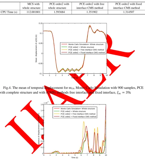
CPU Time (s) 112.001801 1.593684 1.351902 1.314507

Fig.4. The mean of temporal displacement for m19, Monte Carlo Simulation with 900 samples, PCE

with complete structure and with (CMS) methods free interface and fixed interface, 𝜉_𝑚 = 3%

Fig.5. The variance of temporal displacement for m17, Monte Carlo Simulation with 900 samples,

PCE with complete structure and with (CMS) methods free interface and fixed interface𝜉_𝑚 = 3%.

CONCLUSION

The main of this work is to provide the variability of the transient solution of a large and complex structure by considering geometric nonlinearities. We have achieved this by implementing an

0 1 2 3 4 5 6 7 8 9 10

-0.1 -0.05 0 0.05 0.1 0.15 Time (s) M e a n d is p la c e m e n t o f u (1 9 ) (m )

Monte Carlo Simulation+ Whole structure PCE ordre2 + Whole structure PCE ordre2 + Free interface CMS method PCE ordre2 + Fixed interface CMS method

0 1 2 3 4 5 6 7 8 9 10

0 0.2 0.4 0.6 0.8 1 1.2 1.4 1.6x 10

-3 Time (s) v a ri a n c e o f d is p la c e m e n t fo r u (1 9 ) (m 2)

integrated approach, the coupling PCE method, CMS reduction method and temporal integration. The PCE method was used to model the uncertainty parameters, the stochastic solution may be expanded in terms of the polynomial chaos basis whose elements are obtained from Hermit orthogonal polynomial. We developed the CMS method in the nonlinear case for reducing the finite element model. The implementation of the temporal integration by Newmark schema has allowed us to establish the variability of the solution for nonlinear reduced model with uncertain parameters. We could solve the problem of calculating the tangent matrix. The numerical tests show the accuracy of the results and minimization of cost calculation, thus validating this approach.

REFERENCES

[1]. Fishman G. S. Monte Carlo: Concepts, algorithms and Applications. Springer Verlag, 1996.

[2]. Kleiber M, Hien TD. The stochastic finite element method. Ed. Jhon Wiley; 1992.

[3]. Zhao L, Chen Q, Neumann dynamic stochastic finite element method of vibration for structures with stochastic parameters to random excitation, Computers & Structures 2000, 77:651-657.

[4]. Muscolino G, Ricciardi G, Impollonia N, Improved dynamic analysis of structures with mechanical uncertainties under deterministic input. Probabilistic Engineering Mechanics 1999, 15:199-212.

[5]. R.Ghanem, Stochastic finite elements with multiple random non- gaussian properties, J. Eng.

Mech. 60 (4) (1999) 26–40.

[6]. Adhikari S, Manohar C.S, Dynamic analysis of framed structures with statistical uncertainties, International Journal for Numerical Methods in Engineering 1999, 44:1157-1178.

[7]. Li R, Ghanem R, Adaptive polynomial chaos expansions applied to statistics of extremes in nonlinear random vibration, Probabilistic Engineering Mechanics 1998, 125-136.

[8]. Craig RR, Bampton MCC, Coupling of substructures for dynamics analysis, AIAA Journal 1968, 6(7):1313-1319.

[9]. Rubin S, Improved component mode representation for structural dynamic analysis, AIAA Journal 1975, 13(8):995-1006

[10]. Bouhaddi N, Lombard J.P, Improved free interface substructures representation method, Computers & Structures 2000, 269-283.

[11]. MacNeal RH, A hybrid method of component mode synthesis, Computers and Structures 1971, 1:581-601.

[12]. Qiu J, Williams F.W, Qiu R, A new exact substructure method using mixed modes, Journal of Sound and Vibration 2003, 266 : 737–757.

46 10

[14]. Y.Liu, H.Sun, D.Wang, Updating the finite element model of large-scaled structures using component mode synthesis technique, Intelligent Automation and Soft Computing 19 (2013)11– 21.

[15]. C.Papadimitriou, D.C.Papadioti, Component mode synthesis techniques for finite element model updating, Computers and Structures 126(2013) 15–28

[16]. Fritz Adrian Lulf, Duc-Minh Tran, Roger Ohayon , Reduced bases for nonlinear structural dynamic systems: A comparative study, Journal of Sound and Vibration 332 (2013) 3897–3921

[17]. Sarsri D, Azrar L, Jebbouri A, El Hami A, Component mode synthesis and polynomial chaos expansions for stochastic frequency functions of large linear FE models. Computers & Structures 2011, 89:346-356.

[18]. Sarsri D, Azrar L, Time response of structures with uncertain parameters under stochastic inputs based on coupled polynomial chaos expansion and component mode synthesis methods, Mechanics of Advanced Materials and Structures 2016, Vol.23, 5:593-606.