24 INTERNATIONAL JOURNAL OF ADVANCES IN ENGINEERING RESEARCH
ARTIFICIAL NEURAL NETWORK BASED
TOLERANCE ANALYSIS METHOD
*A. Maria Jackson, **Dr. R. Panneer *M. Tech (Advanced Manufacturing), **Associate Professor SASTRA UNIVERSITY, SCHOOL OF MECHANICAL ENGINEERING,
TANJORE, TAMIL NADU, INDIA
ABSTRACT
The following four Tolerance Analysis methods were identified for comparative analysis, critical study and investigation based on the significance of the methods and also considering the versatility of the methods.
(i) SIMULATION BASED STACK-UP ANALYSIS, (ii) SECOND ORDER TOLERANCE ANALYSIS,
(iii) OpTol - SPATIAL TOLERANCE ANALYSIS,
(iv) TOLERANCE ANALYSIS OF 2D AND 3D ASSEMBLIES.
The Literature relevant to the selected methods were critically studied and compiled. Upon gathering further information on the advantages and limitations of these four methods, a framework for the new method will be developed overcoming the problems found in existing methods. Artificial Neural Network will be used to overcome most of the problems found.
Key words – Tolerance Analysis; Simulation; Spatial Tolerance Analysis; Artificial Neural Network.
INTRODUCTION
Tolerance is the total amount that a specific dimension is allowed to vary. Every product is designed with tolerance limits because it is difficult to manufacture component to its exact dimensions because of chance causes and assignable causes of errors. Tolerance is a common arguable point between design and manufacturing. Design Engineer tries to tighten the tolerance for better functionality of the product, whereas Production Engineer tries to relax it for better utilization of resources.
25 INTERNATIONAL JOURNAL OF ADVANCES IN ENGINEERING RESEARCH
METHODOLOGY
As tolerance plays a vital role in success of a industry, it is essential for an Industrial Engineer to understand the world of tolerance. Various methods (about 15) on Tolerance Analysis has been collected for study purposes. Upon study, they are classified into four major types, namely,
o Monte Carlo Simulation (random number for probablity distribution)
o Non Linear Propogation (Develpoment of models to estlabish relationship function) o Computer Aided Tolerance Analysis (Use of a computer software which has a database of
Tolerances).
o 2D and 3D analysis (Creation of vector loops)
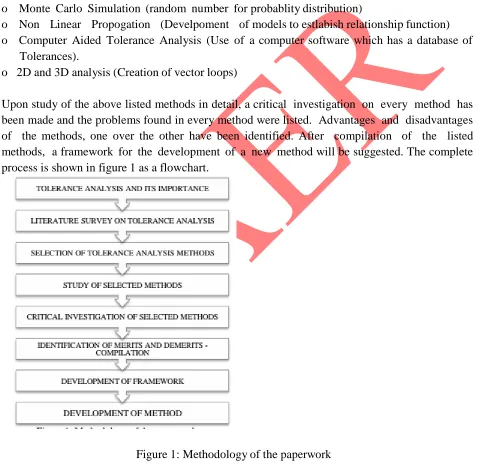
Upon study of the above listed methods in detail, a critical investigation on every method has been made and the problems found in every method were listed. Advantages and disadvantages of the methods, one over the other have been identified. After compilation of the listed methods, a framework for the development of a new method will be suggested. The complete process is shown in figure 1 as a flowchart.
26 INTERNATIONAL JOURNAL OF ADVANCES IN ENGINEERING RESEARCH
INVESTIGATION RESULTS
(i). Number of iterations are variable and it depends on required accuracy level of simulation. Part representation is complex and it depends on size and locations of the sample points. Simulation has its own advantages and disadvantages.
(ii). As quality levels increases sample size increases
100 times. Levelof information required for computation of component tolerance and distribution is high.
(iii). Worst case Tolerance Analysis is rarely encountered in actual manufacturing. Models are assumed to have normal distribution which is not reflected in real conditions.
(iv). Difficulty increases along with the number of chains or loops or chains formed. Evaluation of the vector loop is not discussed.
FRAMEWORK PROPOSAL
A new framework with the objective of overcoming the deficiencies is the objective of the work. As far discussed Simulation is one of the most used yet a deficient step made in tolerance analysis. Artificial Neural Network is the tool proposed here instead of Simulation. Input (Component )tolerances are collected for a particular assembly and functional relationship between input and output assembly tolerances has to be estlabished.
STEP I: For a chosen assembly create the vector loops as stated by Kenneth W. Chase. And find the critical assembly dimension among a particular loop.
STEP II: Now for the number of dimensions and it’s nominal value along with the tolerance values in the particular loop has to be listed.
STEP III: Using Taguchi’s Orthogonal Array construct the table of parameter and response. Vector loop dimensions are parameters with its respective tolerance values as three levels (namely upper, lower and middle values) and closing dimension of vector loop which is the critical dimension of the assembly’s tolerance values is the response of the design. Using Geometric Interpolation the responses can be found using design software.
27 INTERNATIONAL JOURNAL OF ADVANCES IN ENGINEERING RESEARCH
VECTOR LOOP GENERATION
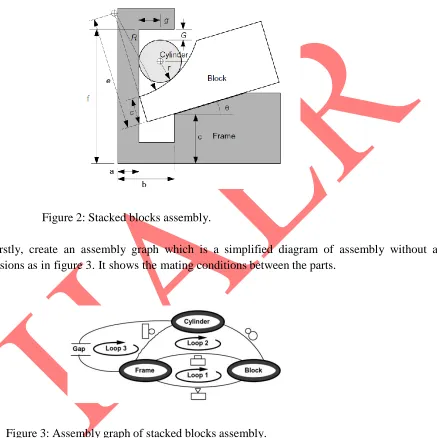
Vector loop generation is explained in steps considering the following assembly shown below in figure 2.
Figure 2: Stacked blocks assembly.
(a) Firstly, create an assembly graph which is a simplified diagram of assembly without any dimensions as in figure 3. It shows the mating conditions between the parts.
Figure 3: Assembly graph of stacked blocks assembly.
28 INTERNATIONAL JOURNAL OF ADVANCES IN ENGINEERING RESEARCH
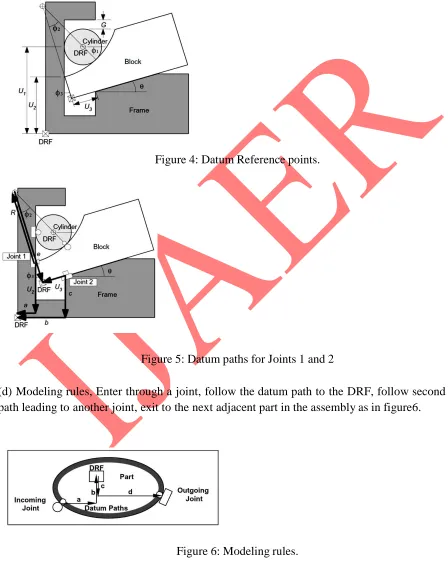
(c) Locate kinematic joints and datum paths. A datum path is a chain of dimensions which locates the point of contact at a joint with respect to a part DRF. Datum paths of the considered assembly is shown in figure 5.
Figure 4: Datum Reference points.
Figure 5: Datum paths for Joints 1 and 2
(d) Modeling rules, Enter through a joint, follow the datum path to the DRF, follow second datum path leading to another joint, exit to the next adjacent part in the assembly as in figure6.
29 INTERNATIONAL JOURNAL OF ADVANCES IN ENGINEERING RESEARCH
NEW METHOD OF TOLERANCE ANALYSIS
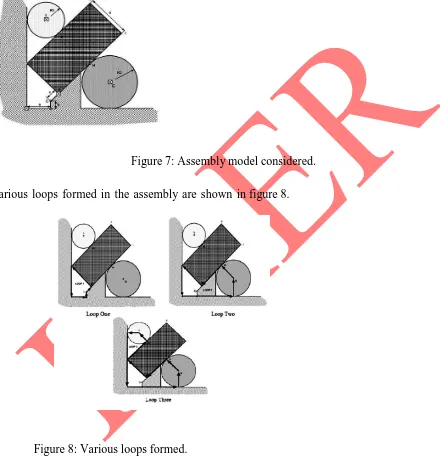
For the new method the assembly considered is shown below in figure 7.
Figure 7: Assembly model considered.
Various loops formed in the assembly are shown in figure 8.
Figure 8: Various loops formed.
30 INTERNATIONAL JOURNAL OF ADVANCES IN ENGINEERING RESEARCH
LOOP I LOOP II LOOP III Name Tol-
Mm Tol+
mm Name Tol- mm
Tol+
mm Name Tol- mm Tol+ mm AB BC CD EA -0.02 -0.02 -0.1 -0.03 0.05 0.01 0.01 0.04 AF FG GH HD DE EA -0.02 -0.05 -0.01 -0.01 -0.05 -0.01 0.02 0 0.01 0.01 0.05 0.04 AF FG GH HD DE EK KL LM MA -0.02 -0.05 -0.01 -0.01 -0.05 0 0 0 -0.02 0.02 0 0.01 0.01 0.05 0 0 0 0.05
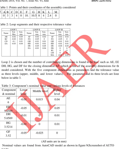
Table 1: Points and their coordinates of the assembly considered Poi
nt nam e
A B C D E F G H K L M
X y coo rds 0 0 3 0 3 1 4 2 0 6 10. 5 0 10.5 3.52 8 6 4 1 0 2.4 2 11. 8 0 11. 8
Table 2: Loop segments and their respective tolerance value
Loop 2 is chosen and the number of contributing dimensions is found to be five, such as AE, ED, DH, HG, and DF for the closing dimension AF, which is one of the assembly dimensions for the model considered. With the five component dimensions as parameters and the tolerance values as three levels (upper, middle, and lower values). The parameter and its three levels are listed below in table 3.
Table 3: Component’s nominal value and various levels of tolerances Component
& nominal
Lower level
Middle level Higher
level AE
6
-0.01 0.015 0.04
ED
5.6569 -0.05 0 0.05
DH 5.6569
-0.01 0 0.01
HG
3.5214 -0.01 0 0.01
GF
3.52 -0.05 -0.025 0
(All units are in mm)
31 INTERNATIONAL JOURNAL OF ADVANCES IN ENGINEERING RESEARCH
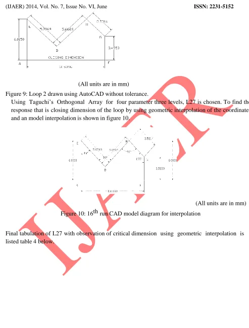
(All units are in mm)
Figure 9: Loop 2 drawn using AutoCAD without tolerance.
Using Taguchi’s Orthogonal Array for four parameter three levels, L27 is chosen. To find the response that is closing dimension of the loop by using geometric interpolation of the coordinates and an model interpolation is shown in figure 10.
(All units are in mm)
Figure 10: 16th run CAD model diagram for interpolation
32 INTERNATIONAL JOURNAL OF ADVANCES IN ENGINEERING RESEARCH
S. No FG 3.52 GH 3.5214 HD 5.6569 DE 5.6569 EA 6 AF (Critical Dimension) 10.52
1 -0.025 0 -0.01 0.05 -0.01 +0.0074
2 -0.025 -0.01 0.01 -0.05 0.04 -0.0648
3 -0.05 0 0.01 -0.05 0.015 -0.0582
4 0 0.01 -0.01 0 -0.01 -0.0299
5 -0.05 -0.01 -0.01 -0.05 -0.01 -0.0667
6 -0.05 0.01 0 -0.05 0.04 -0.0577
7 0 0 0 0 0.04 -0.0299
8 -0.05 0.01 0.01 0 0.04 -0.0155
9 -0.05 -0.01 0.01 0.05 -0.01 0.0127
10 0 0 -0.01 -0.05 0.04 -0.0722
11 0 0.01 0.01 -0.05 -0.01 -0.0441
12 -0.05 0 -0.01 0 0.015 -0.0369
13 -0.025 -0.01 -0.01 0 0.04 -0.0439
14 0 0.01 0 0.05 -0.01 0.0226
15 -0.05 -0.01 0 0 -0.01 -0.0307
16 -0.025 0.01 0.01 0.05 0.015 -0.0196
17 0 -0.01 0.01 0 0.015 -0.0299
18 0 0 0.01 0.05 0.04 0.0125
19 -0.025 -0.01 0 0.05 0.04 -0.0016
20 0 -0.01 0 -0.05 0.015 -0.0722
21 -0.025 0 0 -0.05 -0.01 -0.0591
22 -0.05 0.01 -0.01 0.05 0.04 0.0055
23 -0.05 0 0 0.05 0.015 0.0054
24 -0.025 0 0.01 0 -0.01 -0.0157
25 -0.025 0.01 0 0 0.015 -0.0228
26 -0.025 0.01 -0.01 -0.05 0.015 -0.0642
27 0 -0.01 -0.01 0.05 0.015 -0.0087
Table 4: Final tabulation of interpolated value of critical dimension
33 INTERNATIONAL JOURNAL OF ADVANCES IN ENGINEERING RESEARCH
ARTIFICIAL NEURAL NETWORK
The neural fitting tool (nftool) in Matlab shown in figure 11 is chosen for creating and training the neural network. In nftool window the collected data of component dimensional tolerances as input data and interpolated output dimensional tolerance as output data were fed in excel sheet format. Validation and test data is divided up here in 15% each where the rest 70% of data is used for training the network.
Figure 11: Neural Network fitting tool screenshot.
In network architecture number of hidden neurons was selected by trial and error for better result. Here 10 neurons were chosen. Neural network was created in the next step which has to be trained further. Trained network is plotted for regression in which all the R value has to be closer to one, otherwise retrained. Regression plot of the trained network is shown in figure 12.
34 INTERNATIONAL JOURNAL OF ADVANCES IN ENGINEERING RESEARCH
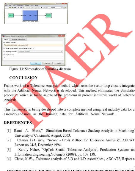
Data are saved and the Simulink diagram was created. In the Simulink diagram the input data were fed for known component dimensional tolerance from which the output assembly tolerance values are generated using the trained neural network. Figure 13 shows the screenshots of Simulink diagram and input parameter blocks.
Figure 13: Screenshot of Simulink diagram.
CONCLUSION
Frame work of a Tolerance Analysis method which uses the vector loop closure integrated with the Artificial Neural Network is developed. This method eliminates the Simulation procedure which is found as one of the problems in present industrial world of Tolerance Analysis.
This framework is being developed into a complete method using real industry data for an assembly and used as the training data for Artificial Neural Network.
REFERENCES
[1] Rami A. Musa,” Simulation-Based Tolerance Stackup Analysis in Machining”, University of Cincinnati, August, 2003.
[2] Charles. G Glancy, ”Second - Order Method for Tolerance Analysis”, ADCATS Report no 94-5, December 1994.
[3] Karoly Nehez, ”OpTol: Spatial Tolerance Analysis”, Production Systems and Information Engineering,Volume 5 (2009), pp. 109-138.
35 INTERNATIONAL JOURNAL OF ADVANCES IN ENGINEERING RESEARCH
99-4, (1999).
[5] Fritz Scholz Research and Technology Boeing Information & Support Services, “Tolerance Stack Analysis Methods”
,December 1995.
[6] K.G.Merkley, K.W.Chase, “An Introduction to Tolerance Analysis”, E. Perry Brigham Young University Provo, UT.
[7] Jirarat, Teeravaraprug, “A Comparative Study of Probabilistic and Worst-case Tolerance Synthesis,” Advance online publication: 12 February 2007, Engineering Letters 14:1, EL_14_1_5.
[8] Polini, Wilma, “A review of two models for tolerance analysis of an assembly: Jacobian and Torsor,” International Journal of Computer Integrated Manufacturing:
04 October 2010 TCIM-2009-IJCIM-0119.R2 [9] Constantinos Mavroidis, “A
REVIEW OF TOLERANCE ANALYSIS OF MECHANICAL ASSEMBLIES,” Department of Mechanical and Aerospace Engineering, Rutgers University.
[10] Kenneth W. Chase, Alan R. Parkinson, “A Survey of Research in the Application of Tolerance Analysis to the Design of Mechanical Assemblies,” Research in Engineering Design (1991) 3:23-37, April 5, 1991
[11] E. E. Lin and H.-C. Zhang, “Theoretical Tolerance Stackup Analysis Based on Tolerance Zone Analysis,” Int J Adv Manuf Technol (2001) 17:257–262.
[12] Gene R. Congano, 2006, Geometric Dimensioning and Tolerancing for Mechanical Design, McGraw-hill
[13] American Society for Quality, “How to perform statistical Tolerance Analysis?”, Volume 11, ISBN 0-87389-010-8, 1986.
[14] Chase, K. W., and W. H. Greenwood, .Design Issues in Mechanical Tolerance Analysis,. Manufacturing Review, ASME, v 1, n 1, pp. 50-59, March, (1988). [15] Ken Chase, ”Basic tools for Tolerance Analysis of mechanical Assemblies” Brigham