METHODOLOGY
Using Gini coefficient to determining
optimal cluster reporting sizes for spatial
scan statistics
Junhee Han
1, Li Zhu
2*, Martin Kulldorff
3, Scott Hostovich
4, David G. Stinchcomb
5, Zaria Tatalovich
2,
Denise Riedel Lewis
2and Eric J. Feuer
2Abstract
Background: Spatial and space–time scan statistics are widely used in disease surveillance to identify geographical areas of elevated disease risk and for the early detection of disease outbreaks. With a scan statistic, a scanning window of variable location and size moves across the map to evaluate thousands of overlapping windows as potential clus-ters, adjusting for the multiple testing. Almost always, the method will find many very similar overlapping clusclus-ters, and it is not useful to report all of them. This paper proposes to use the Gini coefficient to help select which of the many overlapping clusters to report.
Methods: The Gini coefficient provides a quick and intuitive way to evaluate the degree of the heterogeneity of the collection of clusters, which is useful to explain how well the cluster collection reveal the underlying true cluster pat-terns. Using simulation studies and real cancer mortality data, it is compared with the traditional approach for report-ing non-overlappreport-ing clusters.
Results: The Gini coefficient can identify a more refined collection of non-overlapping clusters to report. For exam-ple, it is able to determine when it makes more sense to report a collection of smaller non-overlapping clusters versus a single large cluster containing all of them. It also fulfils a set of desirable theoretical properties, such as being invari-ant under a uniform multiplication of the population numbers by the same constinvari-ant.
Conclusions: The Gini coefficient can be used to determine which set of non-overlapping clusters to report. It has been implemented in the free SaTScan™ software version 9.3 (www.satscan.org).
Keywords: Scan statistic, SaTScan, Cluster detection, Cancer mortality, Log likelihood ratio, Cluster reporting size, Gini coefficient, Spatial statistics, Disease surveillance
© 2016 The Author(s). This article is distributed under the terms of the Creative Commons Attribution 4.0 International License (http://creativecommons.org/licenses/by/4.0/), which permits unrestricted use, distribution, and reproduction in any medium, provided you give appropriate credit to the original author(s) and the source, provide a link to the Creative Commons license, and indicate if changes were made. The Creative Commons Public Domain Dedication waiver (http://creativecommons.org/ publicdomain/zero/1.0/) applies to the data made available in this article, unless otherwise stated.
Background
Spatial and spatio-temporal scan statistics play an increasingly important role in public health surveil-lance. Cluster-detection tools based on these statistics have been broadly utilized in identifying geographic patterns and clusters of chronic diseases [1], detect-ing outbreaks of communicable diseases [2, 3], as well as linking possible risk factors to disease outcomes [4].
A likelihood-based approach allows the scan statistic to identify clusters and evaluate if they are statistically sig-nificant, adjusting for the multiple testing inherent in the many potential cluster locations and sizes.
A variable sized candidate area (scanning window) lit-erally scans across the study region. For each window, the likelihood is calculated and the candidate area with the maximum likelihood defines the most likely cluster. Several methods have been proposed in this class. This includes circular and elliptic spatial scan statistics [5, 6], as well as non-parametric spatial scan statistics that aim to detect irregular shaped cluster. The latter are non-parametric in terms of the spatial cluster shapes, not in
Open Access
*Correspondence: [email protected]
2 Surveillance Research Program, Division of Cancer Control
and Population Sciences, National Cancer Institute, National Institutes of Health, Bethesda, MD 20892, USA
terms of the likelihood functions, and they include e.g. Duczmal and Assunção’s [7] simulated annealing scan statistic, Tango’s [8] flexibly shaped spatial scan statistic, Patil and Taillie’s [9] upper-level set scan statistic, Gang-non and Clayton’s [10, 11] likelihood-based method, Costa et al.’s [12, 13] spanning tree scan statistics, and Duczmal et al.’s [14] genetic algorithm scan statistic.
Many studies have been conducted on the statistical power of scan statistics with predefined varying shapes and sizes. As one would intuitively expect, the circular spatial scan statistic has best power for compact clusters while non-parametric scan statistics have best power for irregularly shaped clusters [15–19]. Specifically, Huang et al. [17] performed an intensive simulation study on power and sample size requirements for tests with differ-ent spatial patterns in terms of geographic locations and relative risks. They found that the elliptic version per-forms well for cluster detection in data with a variety of spatial patterns. Based on their findings, we focus on the elliptic purely spatial scan statistic but the principles and theory described here applies to other likelihood-based methods and the space–time scan statistics as well.
The spatial scan statistic requires a maximum spatial window size (MSWS). In the SaTScan™ software, this can be defined based on the size of the population or the geo-graphic area of the study region. The maximum spatial window size is often defined to be less than or equal to 50 % of the total population at risk (Table 1). Ribeiro and Costa [20, 21] explored different values for the maximum cluster size and suggested that performance is sensitive to the maximum cluster size chosen by the user. This is natural. With a larger maximum, a much larger set of potential clusters are evaluated, so there is more multi-ple testing to adjust for. More importantly, with a smaller maximum, larger clusters are not evaluated and cannot therefore be found. A general guideline is to select the maximum so that any clusters larger than that maximum is of no public health interest. While it has sometimes been done (Table 1), one should never run the analysis multiple times using different values for the maximum. If that is done, then those analyses performed with a smaller maximum will not adequately adjust for the
multiple testing that was done when also evaluating the larger clusters. If multiple maxima were used by mistake, one should report the p values from the largest maximum used.
When rejecting the null hypothesis in a spatial scan statistic analysis, there are almost always multiple sta-tistically significant clusters that overlap each other and the number can be in the thousands. While the SaTScan software can provide all of these overlapping clusters, it is not meaningful to report all of them, since many of them are almost identical. As the default, SaTScan has reported clusters hierarchically, first reporting the clus-ter with the maximum likelihood, and then reporting the one with the maximum likelihood among the remaining clusters that do not overlap an already reported cluster. When using a large maximum window size, the maxi-mum likelihood will sometimes be obtained for a large cluster that contains several smaller clusters, and it is not always clear whether it is better to report one large cluster or several smaller ones. The decision on which collection of clusters better represents the underlying patterns is currently very subjective due to a lack of sys-tematic ways to evaluate the cluster models. Specifically, as we will see later, the hierarchical approach may turn up with unnecessarily large and less informative clusters. Within a pre-determined maximum cluster size such as 50 % of the population at risk, the goal of the Gini coef-ficient, which we propose in this paper, is to determine the best collection of non-overlapping statistically signifi-cant clusters to report, from among the many thousands of statistically significant and highly overlapping clusters that the spatial scan statistic finds.
Most likely cluster and statistical inference
Suppose we have a geographical region partitioned into sub-regions such as counties or census tracts. The areas are represented either by their geometrical or population weighted centroids using the longitude and latitude coor-dinates, their age and gender specific population at risk, and the number of cancer cases in each area. Centered at each centroid, the spatial scan statistic uses a very large collection of overlapping circles of continuously varying
Table 1 Selection of maximum spatial window size in 81 recent publications
Using Google Scholar, we ran a search of publications with both words “SaTScan” and “cancer” published during 2015 and yielded 156 results. Restricting the search to scientific papers published in peer-reviewed journals in English, we found a total of 81 papers using the SaTScan™ software (www.satscan.org). This table summarizes the maximum spatial window size (MSWS) used in these 81 papers. 8 papers (10 %) erroneously (see reason in “Maximum spatial window size of reported clusters” section) used multiple MSWS ranging from 2 to 4 choices, with 50 % always included as one of them
Maximum spatial window size <5 % 10 % 15 % 25 % 30 % 50 % Multiple maxima Distance based Not specified Total
# of pub. 5 3 1 5 1 22 8 13 23 81
radius to define a set of potential clusters. Alternatively, the method uses a collection of ellipses with continuously varying lengths and widths for a predefined set of shapes and directional angles. An MSWS is defined in terms of geographical area or as a percentage of total population at risk. To define a cluster, the maximum is never chosen as more than 50 % of the total population at risk.
Let Z be the collection of all the geographic units in study region S. Zone z consists of neighboring geo-graphic units (e.g. counties) and can have varying shapes and sizes. Let cz and nz be the observed number of cases and the expected number of cases (or population) in zone z, respectively. Then C=zcz and N=znz will be the total number of cases and the total number of expected cases in S. For cancer incidence and mortality, a Poisson model is typically chosen. The likelihood ratio [5] of a zone z is then given by
If there is interest in scanning for ‘negative clusters’ with a lower rate than expected, the indicator func-tion is replaced by I(cz < nz) and if the interest is in clusters of both higher and lower rates, the indicator function is removed. It is equivalent but numerically easier to work with the logarithm, and the test statistic is T =maxzlog(LR(z))=maxzLLR(z). That is, the most likely cluster is the scanning window z ∈ Z, which maxi-mizes the log likelihood ratio.
The test statistics T follows approximately an extreme value distribution [22, 23], but the exact distribution is unknown, so statistical significance is evaluated using Monte Carlo hypothesis testing. This is done by creat-ing a large number of random data sets generated under the null hypothesis that there is no cluster, and calculat-ing the value of the test statistic for each of those random data sets. The Monte Carlo p value is then calculated as r/ (1 + m) where r is the rank of the test statistic from the real data set among all the random data sets and m is the number of random data sets. For example, with a statis-tical significance level of α = 0.05, the cluster will cause a rejection of the null hypothesis if its likelihood ratio is within the highest 5 % among all the maximum likeli-hood ratio from the one real and the m random data sets. Calculations were performed using SaTScan™ version 9.3.
Secondary clusters
In addition to the most likely cluster, it is also of inter-est to know if there are additional clusters present in the data. The secondary clusters in the real data are also compared to the most likely clusters in the random data
(1) LR(z)=
cz nz
cz C−cz N−nz
C−cz
I(cz>nz)
sets. In this way, they are only statistically significant if they can reject the null hypothesis on their own strength, irrespective of whether the more likely clusters are true clusters or not. Most secondary clusters overlap with and some only differ slightly with a more likely cluster. While these secondary clusters are always evaluated as part of an analysis, it is not meaningful to report all of them. The SaTScan software has several options on how to report overlapping clusters. In version 9.1 and earlier, the default was a hierarchical option of only reporting clus-ters that do not overlap with an already reported more likely cluster. A consequence of this is that a large most likely cluster can hide several smaller distinct clusters, and the hierarchical approach is not necessarily the best way to select a set of non-overlapping clusters to report.
Maximum spatial window size of reported clusters
Since the spatial scan statistic evaluates clusters of differ-ent window sizes, it is critically important to adjust for the multiple testing generated by all the different window sizes considered. This means that it is incorrect to run the scan statistic multiple times with different values for the MSWS, and then select the clusters with the lowest p value. When doing so, one does not properly adjust for all the multiple testing conducted, and the p values will be biased. It is not always the most likely cluster that is of primary importance though, and a set of smaller sub-clusters can sometimes be of greater interest. It is per-fectly fine to report only those and their corresponding p values, as long as proper multiple testing adjustment is made for all the smaller and larger clusters that were also evaluated in the analysis. One way to do this in the SaTScan software is to rerun the analysis and request that it only report clusters of a certain maximum size, while still adjusting for the multiple testing inherent in all the sizes considered in the other prior analyses of the same data, by keeping the MSWS fixed at a larger value. This is an advanced feature in the SaTScan software, and mul-tiple analyses can be done repeatedly on the same data with the same fixed MSWS (e.g. 50 %) but with different maximum reported cluster sizes (MRCS, e.g. 5, 10, 20, and 50 %).
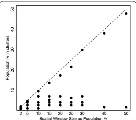
As the sizes of reportable clusters increases, SaTS-can often reports a bigger cluster with a size close to the MRCS rather than clusters of smaller or medium size. This is because two or three small clusters close to each other may have a larger likelihood when combined into one big cluster even if there are few observed cases in between the clusters. An example is given in Figs. 1 and
[25]. In both Figures, SaTScan is run with the MRCS at various levels expressed as percentage in the population. Under each user-provided MRCS, clusters are reported in SaTScan and presented here. Figure 1 shows the MRCS (expressed as a percentage in population) as the horizontal axis. The vertical axis represents the percent-age of population in each reported cluster, over the total U.S. female population in 2006. The dashed line is the ref-erence that the percentage of cluster population equals to the MRCS. Each dot represents a cluster detected at the corresponding MRCS. Figure 2 selects four levels of MRCS, i.e., MRCS = 2, 15, 25, and 50 % of population, and maps the clusters detected at the corresponding MRCS. Each cluster is illustrated with a difference colour and the relative risk (RR) is labelled on the cluster. When the MRCS is restricted at 2 % of population, SaTScan detects a total of 16 clusters with RR ranging between 1.18 and 2.81 (Fig. 2). Every cluster has a population below the level of MRCS, i.e. 2 % of the total popula-tion (Fig. 1). When the MRCS increases, smaller clusters merge into larger ones and the RR’s in the larger clusters tend to be smaller as more and more areas are merged into them. When the MRCS is set at the SaTScan default of 50 % of population, a cluster that accounts for 47 % of U.S. female population is detected with RR of 1.2, along with a small cluster in the northwest of U.S. with RR of 1.24. Figure 1 also shows that at each level of the MRCS, SaTScan always reports a large cluster with the percent-age of population very close to the level of MRCS, and the smaller clusters are simply merged into larger ones when the MRCS increases. This observation is true not
only for female lung cancer mortality but also for many other cancer sites that we examined, including female breast cancer, prostate cancer, ovary cancer, bladder can-cer, and cervical cancer (data not shown), although obvi-ously not for all data sets.
With the Gini coefficient, we will try to find a suitable and informative collection of non-overlapping clusters to report, avoiding overly large clusters with relatively small RR (such as the cluster with 47 % of population and RR = 1.2), as well as many tiny clusters that may blur the big picture of the geographic pattern. The proposed methods in this paper will help to identify clusters with meaningful RR as well as distinct geographic distribution pattern.
An important question is whether there is more evi-dence for a few larger clusters or several smaller ones. Another question is which clusters to present in a pub-lic health or epidemiological research study, if we only want to report non-overlapping clusters. In this paper, we propose a criterion for selecting a set of non-overlapping clusters to report based on the Gini coefficient. Findings from both simulated data and real cancer mortality data show that the Gini coefficient is able to determine when it makes more sense to report a collection of smaller non-overlapping clusters versus a single large cluster con-taining all of them. It will sometimes avoid overly large clusters with relatively small relative risk (RR), such as the cluster with 47 % of population and RR = 1.2, in favour of a few smaller clusters with higher RR. Compared to using a small MRCS, it will sometimes avoid reporting many tiny clusters that may blur the big picture of the geo-graphic pattern.
Methods
Lorenz curve and Gini coefficient
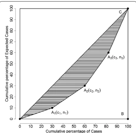
In economics, the Lorenz curve [26] is often used to explain and measure the heterogeneity of the wealth dis-tribution. It is a graphical representation of the cumulative distribution function of the empirical probability distri-bution. The basic format of the graph is a square divided into two symmetric isosceles right triangles (as illustrated in Fig. 3). In this illustration, point Ai(ci, ni) denotes that the bottom ni % of population own ci % of total wealth and point Ai’s are ordered so that the ni are in non-decreasing order. Line OC in the triangle (line y = x) depicts a per-fectly equal wealth distribution and is used as the refer-ence line. The two legs of the triangle, OB and BC, depict the perfectly unequal wealth distribution, i.e., no house-hold owns any wealth except for the very last one which owns all the wealth in the whole society. Curve OA1A2A3C inside the triangle is called the Lorenz curve and describes the observed wealth distribution. The Lorenz curve is then compared to the reference line OC, the line for the
perfectly equal wealth distribution. The Gini coefficient [27, 28] is a common measure to describe the behaviour of the Lorenz curve. It is simply the ratio of the areas OA1A2A3C and OBC. Since area OBC accounts for ½ of the whole square, the denominator in the Gini coefficient is often taken as ½, hence the value of the Gini coefficient of a Lorenz curve is two times the shaded area. The Lor-enz curve and Gini coefficient were originally developed to measure wealth inequality, and have been extended in the area of health disparity in the recent decade. [29–31].
Here we apply the methods of the Lorenz curve and the Gini coefficient to describe collections of disease clusters. If there is a significant cluster in the study region, then the distribution of disease cases tends to be concentrated in the cluster, pushing the Lorenz curve further away from the reference line, and the value of the Gini coeffi-cient will be higher. In Fig. 3, the cumulative percentages of expected cases are on the x-axis and the cumulative percentages of diseases (for example, new cases from cancer) are on the y-axis. The reference line is present-ing a perfect equality (or randomness) in the distribution of the deaths, when the cumulative percentages of new cases are exactly the same as the cumulative percent-ages of the expected cases, i.e. there are no statistically significant clusters. When comparing several competing
collections of non-overlapping clusters, the one with the highest Gini coefficient value should be chosen as the cluster collection to report.
Fig. 2 Spatial clusters and the relative risks at various maximum spatial window sizes (U.S. Female Lung Cancer Mortality, 2006; Clusters are identi-fied in colour with relative risks labelled on clusters.)
In the illustration of Fig. 3, the x- and y-axes repre-sent the cumulative percentages of observed cases and expected cases, respectively. Each cluster Ai has coordi-nates (ci, ni). The origin point O’s coordinates are (0, 0) and point C has coordinates (cI+1, nI+1) = (1, 1). The
rela-tive risk for cluster Ai is calculated as nici−−ci−ni−11. The clusters
are sorted so that the relative risks of cluster Ai’s are non-increasing. Note that
and
By definition, the Gini coefficient is two times of the shaded area, and can be expressed as
where c0=n0=0 and cI+1=nI+1=1. With some
alge-bra, Gini coefficient can also be expressed as
Theoretical features of Gini coefficient
The value of the Gini coefficient is between 0 and 1, with higher values indicating higher disparity in the clus-ters. In selecting clusters to report, the cluster set with the highest Gini coefficient value is picked. A nice prop-erty of the Gini coefficient is that it is unchanged if the population in all locations are multiplied by the same constant. There are four other important theoretical fea-tures that we think that any reasonable selection criterion should have, and we show that the Gini coefficient satis-fies all of them. The four features can be expressed as: (1) If two sets of clusters have the same number of clusters and same expected number of cases, the set with more cases should be selected; (2) If two sets of clusters have the same number of clusters, and one set has more cases and expected cases than the other and the excess num-ber is the same for both cases and expected cases, then one should select the cluster set with fewer expected cases; (3) If one set of clusters contain all the clusters in the other set, then the set with more clusters should be selected; and (4) If one set has fewer clusters than the other but the total number of cases and expected cases are the same for the two clusters, the set with fewer clus-ters should be selected.
To prove that Gini coefficient has all the four features, the following notation is used. Two sets of clusters, set 1 and set 2, are being considered, with the number of
(2)
ci≥ni
(3)
ci−ci−1
ni−ni−1
≥ ci+1−ci ni+1−ni
(4)
G=1−
I+1
i=1
(ni−1+ni)(ci−ci−1)
(5)
G=
I+1
i=1
(nici−1−ni−1ci)
clusters being I1 and I2, respectively. In each cluster i,
the number of expected cases are ni,1 and ni,2, and the number of observed cases are ci,1 > ni,1 and ci,2 > ni,2. The Gini coefficients are G1 and G2 for cluster set 1 and set 2
respectively. Here we will show that the Gini coefficient satisfies the following theoretical criteria.
Theorem 1 If I1 = I2 = I, ni,1 = ni,2 = ni for all i, ci,1 ≥ ci,2 for all i, and ci,1 > ci,2 for at least one i, then G1>G2. This criterion guarantees that when comparing two sets of clusters with the same number of clusters and the same expected counts, the set with uniformly more cases is selected to be reported.
Proof It can be shown that the difference in the Gini coefficients for the two sets of clusters, G1 and G2, is cal-culated as
Using similar algebra, we can prove the following fea-tures are also true for Gini coefficients.
Theorem 2 If I1 = I2, ni,2 = ni,1 + k and ci,2 = ci,1 + k for all i, and k ≥ 0, then G1≥G2. This feature means that when comparing two sets of clusters with the same excess count (ci − ni), the selection rule will favour the set with the smaller expected counts.
Theorem 3 If I1 > I2, ni,j=n and ci,j=c for all clusters
i in both sets j, then G1>G2. This criterion means that if there are multiple identical clusters in the two sets to be considered, the one with more clusters will be picked.
Theorem 4 If I1≤I2, I1
i=1ci,1 = I2i=1ci,2 and
I1
i=1ni,1=
I2
i=1ni,2, then G1≥G2. This criterion states
that if there are multiple clusters, and they can be joined into a fewer number of clusters without adding anything else, then the set with the joined clusters is preferred.
Data and simulation examples
In order to evaluate the performance of the Gini coef-ficient, we use both actual cancer mortality data and simulated data on selected cancer sites. To gain a com-plete understanding of the performance of the proposed
G1−G2= I+1
i=1
[(ni,1ci−1,1−ni−1,1ci,1)−(ni,2ci−1,2−ni−1,2ci,2)]
= I+1
i=1
[(nici−1,1−ni−1ci,1)−(nici−1,2−ni−1ci,2)]
= I+1
i=1
criteria, we select cancer sites of various levels of fre-quency. For rare cancers, the total number of deaths in a single year will be too small to produce reliable estimates of relative risks, so multiple years of data are aggregated to mitigate this problem. Table 2 lists the selected can-cer sites, the total number of deaths for these cancan-cers in year 2006, and the time span the mortality data are aggre-gated. In addition to the actual cancer mortality data, for each cancer site, simulated data are created to evaluate the proposed criterion. The simulated cancer mortality data are created based on the Gini chosen clusters for the actual mortality data, with the same level of relative risks for the clusters.
The other simulated data are from the Northeastern USA benchmark data sets published on the SaTScan website www.satscan.org/datasets.html and described in detail before [15]. We use several simulated data sets from this source with both 600 and 6000 cases. Three different sets of local clusters are constructed in a rural, urban, and mixed urban/rural area respectively. Within each of these three sets, cluster sizes vary with 1, 2, 4, 8, and 16 counties respectively. The data sets rural, urban and mixed contain single hot-spot clusters around Grand Isle, New York City, and Pittsburgh respectively.
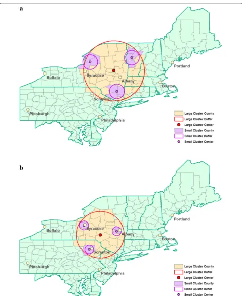
In situations that one big cluster or several small clus-ters exist in a study area, the hierarchical way of report-ing clusters in SaTScan will usually detect one big cluster in both situations when 50 % is set as the maximum spa-tial window size. The Gini coefficient may perform better and settle on one big cluster in the first case and a few smaller ones in the other. To evaluate this, the third sim-ulated data is created using the same geographical area as the Northeastern USA benchmark data. Large and small clusters are created in the same area, as shown in Fig. 4. Configuration A (urban center with small rural clus-ters) consists of a large cluster of counties with an urban area in its center (Albany, NY) and three smaller clus-ters within the same area that consist of rural counties.
Configuration B (rural center with small urban clusters) consists of a large cluster of counties with a rural area in its center and three smaller clusters within the same area that consist of urban counties (Albany, NY, Syracuse, NY, and Scranton, PA).
Results
Table 3 shows the optimal maximum reported cluster size (MRCS) chosen based on the Gini coefficient for both actual and simulated cancer mortality data. The clusters reported with either the best MRCS, or the second best MRCS when a 50 % MRCS is identified as the optimal, are used to create the simulated data. The second best MRCS is shown in parentheses under the “Actual Data” column. With the total number of cases fixed as in Table 2, we generate simulated datasets for each of the eight cancer sites. For male lung cancer mortality, Gini reports 50 % as the optimal MRCS, and the second best MRCS is of size 10 %. The simulated male lung cancer mortality data is then created using the cluster model reported at the 10 % MRCS level. Gini coefficient correctly identifies 10 % as the optimal MRCS for the simulated data. For the actual female lung cancer mortality data in 2006, Gini coefficient picks 15 % as the optimal MRCS. In the simu-lated female lung cancer mortality data, Gini coefficient correctly identifies 15 % as the optimal MRCS as well. Actually, the Gini coefficient always identifies the cor-rect MRCS for all the eight simulated data in Table 3. For actual female lung cancer mortality data in 2006, Fig. 5
plots the value of Gini coefficient at the various MRCS levels. MRCS with the highest Gini value, at 15 % of pop-ulation, is the optimal cluster reporting size.
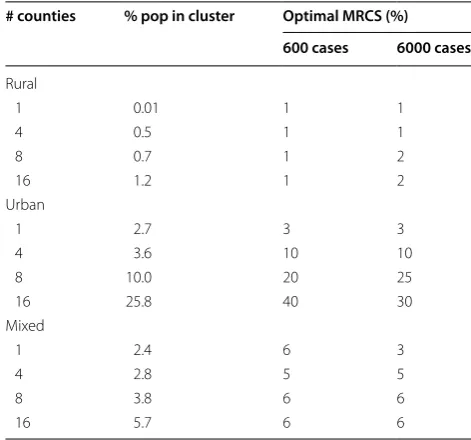
Another simulation study is based on the Northeast-ern USA benchmark data sets. Data sets rural, urban, and mixed contain one cluster in a rural, urban, or mixed urban/rural area, respectively. Table 4 shows the optimal MRCS determined by the Gini coefficient values using the Northeastern USA Benchmark data with either 600 or 6000 total cases. As shown in the table, as the num-ber of counties in the cluster increases, the percent of population in the “true” cluster increases, and the MRCS picked by the Gini coefficient varies, depending on the location of the cluster. If the true cluster is located in a rural area, then the MRCS required to pick the right clus-ter is 1 or 2 % in most cases, because the percentage of population in the true cluster is always below 2 %. If the true cluster is in an urban area, then as the number of counties increase in the cluster, so does the population in the cluster (from 2.7 to 25.8 % of all the population in the study area). The optimal MRCS increases from 3 to 40 % in the scenario of 600 cases and from 3 to 30 % in the sce-nario of 6000 cases. If the true cluster is located in a mix of rural and urban areas, the optimal MRCS remains in
Table 2 Cancer sites of the actual US cancer mortality data, 2006
Cancer site Total number
of deaths Years of data aggregation
Lung, male 88,791 2006
Lung, female 69,037 2006
Breast 40,600 2006
Prostate 28,256 2006
Ovary 14,781 2002–2006
Bladder, male 9368 2000–2006
Bladder, female 4049 2000–2006
the level close to the percent of population in the true cluster. In the case of two or multiple clusters (data not shown), there is not much difference in the MRCS as the number of counties increase in the cluster.
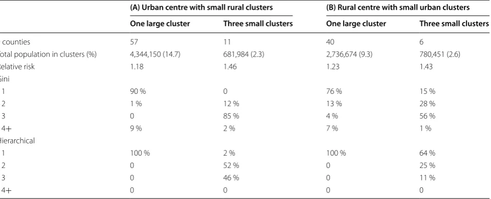
In the third simulation study, we examine the behavior of the Gini coefficient when a large cluster or three small clusters exist in the same regions. The hierarchical way of reporting clusters in SaTScan will more likely report the single large cluster in both situations, while the Gini coefficient can identify the correct large or small clusters more often. Table 5 presents the details of the simulated data, which includes number of counties, the population
size, percent of population over the study area, and rela-tive risk in each of the large or small clusters in the two configurations described in Fig. 4. The relative risks are calculated using the algorithm in Kulldorff [15] to guar-antee a statistical power of 0.999 under the alternative hypothesis of significant disease clusters. A total of 1000 replications of each configuration are created. Table 5
shows that for the Gini coefficient and the SaTScan hier-archical approach, what percent of the 1000 replications report 1, 2, 3, or 4+ clusters in each of the “One Large Cluster” or “Three Small clusters” scenarios. A better criterion will show higher percentage for 1 cluster in the “One Large Cluster” columns and 3 clusters in the “Three Small clusters” columns. If only one large cluster exists, in both urban center and rural center scenarios, the SaTS-can hierarchical approach always identifies 1 large cluster, while Gini detects 1 large cluster 90 % of the time in the urban center and only 76 % of the time in the rural center. When 3 small clusters exist, SaTScan correctly detects 3 small clusters 46 % of the time in the urban center and only 11 % of the time in the rural center scenarios. Gini coefficient outperforms the hierarchical approach with 85 and 56 % correct reporting respectively. While the hier-archical approach does slightly better when there is one large cluster, the Gini coefficient does a lot better when there are many small clusters. Generally, Gini coefficient tends to report smaller multiple clusters while the hierar-chical approach tends to report fewer and larger clusters.
Table 3 Optimal maximum reported cluster size (MRCS, in percent of population) chosen by the Gini coefficient for actual cancer mortality data and simulated cancer mor-tality data
a Numbers in parentheses are the second best MRCS chosen by Gini coefficient
Cancer site Year(s) Actual dataa Simulated data
Male lung 2006 50 (10) 10
Female lung 2006 15 (10) 15
Breast 2006 30 (25) 30
Prostate 2006 10 (2) 10
Ovary 2002–2006 25 (30) 25 Male bladder 2000–2006 5 (10) 5 Female bladder 2000–2006 50 (15) 15 Cervical 2000–2006 5 (10) 5
Fig. 5 Values of Gini and CLIC at various maximum spatial window sizes for U.S. Female Lung Cancer Mortality, 2006
Table 4 Optimal MCRS identified by the Gini coefficient in the Northeastern USA benchmark data
# counties % pop in cluster Optimal MRCS (%)
600 cases 6000 cases
Rural
1 0.01 1 1
4 0.5 1 1
8 0.7 1 2
16 1.2 1 2
Urban
1 2.7 3 3
4 3.6 10 10
8 10.0 20 25
16 25.8 40 30
Mixed
1 2.4 6 3
4 2.8 5 5
8 3.8 6 6
Discussion
The spatial scan statistic will almost always find multi-ple overlapping statistically significant clusters, and it is not useful to report all of them. Some users have uti-lized multiple different maximum spatial window sizes (MSWS) in an attempt to find most important clusters, but that is invalid from a statistical perspective since it does not appropriately account for the multiple test-ing. Keeping the MSWS fixed, it is valid to try different maximum reported cluster sizes (MRCS), but there has not been an objective criterion for deciding which collec-tion of clusters to present. In practice, the MRCS is either determined arbitrarily in an ad-hoc manner or set at 50 % of the population. We found that setting MRCS at 50 % often results in unnecessarily large and less informative clusters.
Conclusions
We propose to use the Gini coefficient as a more intui-tive and systematic way to determine the best collec-tion of clusters to report. It is not intended to evaluate the statistical significance of disease clusters; instead, it is developed to select a suitable and informative collec-tion of non-overlapping cluster to report, among the many overlapping clusters identified by the spatial scan statistics. Hence, instead of replacing the spatial scan sta-tistics, Gini coefficient enhances the spatial scan statistics by providing a criterion to select the collection of non-overlapping clusters to report. It identified the correct clusters in simulation studies and performed better than the hierarchical cluster reporting option. It also has the important property of being invariant under a uniform
multiplication of the population numbers by the same constant. Gini coefficient is also shown to satisfy other important theoretical features.
The Gini coefficient has been implemented in the free SaTScan™ software version 9.3 (www.satscan.org).
Abbreviations
MRCS: maximum reported cluster size; MSWS: maximum spatial window size.
Author details
1 Division of Biostatistics, Research Institute of Convergence for Biomedical
Science and Technology, Pusan National University Yangsan Hospital, Pusan, Korea. 2 Surveillance Research Program, Division of Cancer Control and
Popula-tion Sciences, NaPopula-tional Cancer Institute, NaPopula-tional Institutes of Health, Bethesda, MD 20892, USA. 3 Brigham and Women’s Hospital and Harvard Medical School,
Boston, MA, USA. 4 Information Management Services, Calverton, MD, USA. 5 Westat, Inc, Rockville, MD, USA.
Authors’ contributions
JH, LZ, MK DGS, ZT, DRL, and EJF developed the method and study design. MK and SH implemented the method in SaTScan. JH and LZ carried out the analyses. JH, LZ and MK drafted the manuscript. All authors read and approved the final manuscript.
Acknowledgements
The authors acknowledge two anonymous peer reviewers who have provided comments that improved the quality of this manuscript.
Competing interests
The authors declare that they have no competing interests.
Availability of data and material
The software along with datasets supporting the conclusions of this article are included as supporting materials.
Funding
This work was partly supported by the Statistical Methodology and Applica-tions Branch of the National Cancer Institute through an Intergovernmental Personnel Act (JH).
Table 5 Comparison of the Gini coefficient and the hierarchical cluster reporting criteria using the simulated cluster con-figurations in the Northeastern USA
(A) Urban centre with small rural clusters (B) Rural centre with small urban clusters
One large cluster Three small clusters One large cluster Three small clusters
# counties 57 11 40 6
Total population in clusters (%) 4,344,150 (14.7) 681,984 (2.3) 2,736,674 (9.3) 780,451 (2.6)
Relative risk 1.18 1.46 1.23 1.43
Gini
1 90 % 0 76 % 15 %
2 1 % 12 % 13 % 28 %
3 0 85 % 4 % 56 %
4+ 9 % 2 % 7 % 1 %
Hierarchical
1 100 % 2 % 100 % 64 %
2 0 52 % 0 25 %
3 0 46 % 0 11 %
• We accept pre-submission inquiries
• Our selector tool helps you to find the most relevant journal • We provide round the clock customer support
• Convenient online submission • Thorough peer review
• Inclusion in PubMed and all major indexing services • Maximum visibility for your research
Submit your manuscript at www.biomedcentral.com/submit
Submit your next manuscript to BioMed Central
and we will help you at every step:
Received: 15 June 2016 Accepted: 20 July 2016
References
1. Kulldorff M, et al. Breast cancer clusters in the northeast United States: a geographic analysis. Am J Epidemiol. 1997;146(2):161–70.
2. Lee SS, Wong NS. The clustering and transmission dynamics of pandemic influenza A (H1N1) 2009 cases in Hong Kong. J Infect. 2011;63(4):274–80. 3. Huang SS, et al. Automated detection of infectious disease outbreaks in
hospitals: a retrospective cohort study. PLoS Med. 2010;7(2):e1000238. 4. McNally RJ, Ducker S, James OF. Are transient environmental agents
involved in the cause of primary biliary cirrhosis? Evidence from space– time clustering analysis. Hepatology. 2009;50(4):1169–74.
5. Kulldorff M. A spatial scan statistic. Commun Stat Theory Methods. 1997;26(6):1481–96.
6. Kulldorff M, et al. An elliptic spatial scan statistic. Stat Med. 2006;25(22):3929–43.
7. Duczmal L, Assuncao R. A simulated annealing stratergy for the detection of arbitrarily shaped spatial clusters. Comput Stat Data Anal. 2004;45(2):269–86.
8. Tango T, Takahashi K. A flexibly shaped spatial scan statistic for detecting clusters. Int J Health Geogr. 2005;4:11.
9. Patil GP, Taillie C. Upper level set scan statistic for detecting arbitrarily shaped hotspots. Environ Ecol Stat. 2004;11(2):183–97.
10. Gangnon RE, Clayton MK. Likelihood-based tests for localized spatial clustering of disease. Environmetrics. 2004;15(8):797–810.
11. Gangnon RE, Clayton MK. A weighted average likelihood ratio test for spatial clustering of disease. Stat Med. 2001;20(19):2977–87.
12. Assuncao R, et al. Fast detection of arbitrarily shaped disease clusters. Stat Med. 2006;25(5):723–42.
13. Costa MA, Assuncao RM, Kulldorff M. Constrained spanning tree algo-rithms for irregularly-shaped spatial clustering. Comput Stat Data Anal. 2012;56(6):1771–83.
14. Duczmal L, et al. A genetic algorithm for irregularly shaped spatial scan statistics. Comput Stat Data Anal. 2007;52(1):43–52.
15. Kulldorff M, Tango T, Park PJ. Power comparisons for disease clustering tests. Comput Stat Data Anal. 2003;42(4):665–84.
16. Song C, Kulldorff M. Likelihood based tests for spatial randomness. Stat Med. 2006;25(5):825–39.
17. Huang L, Pickle LW, Das B. Evaluating spatial methods for investigat-ing global clusterinvestigat-ing and cluster detection of cancer cases. Stat Med. 2008;27(25):5111–42.
18. Kulldorff M, et al. Benchmark data and power calculations for evaluating disease outbreak detection methods. MMWR Morb Mortal Wkly Rep. 2004;53(Suppl):144–51.
19. Duczmal L, Kulldorff M, Huang L. Evaluation of spatial scan statistics for irregularly shaped clusters. J Comput Graph Stat. 2006;15(2):428–42. 20. Ribeiro SH, Costa MA. Optimal selection of the spatial scan parameters
for cluster detection: a simulation study. Spat Spatiotemporal Epidemiol. 2012;3(2):107–20.
21. Chen J, et al. Geovisual analytics to enhance spatial scan statistic inter-pretation: an analysis of U.S. cervical cancer mortality. Int J Health Geogr. 2008;7:57.
22. Abrams AM, Kleinman K, Kulldorff M. Gumbel based p-value approxima-tions for spatial scan statistics. Int J Health Geogr. 2010;9:61.
23. Jung I, Park G. p-value approximations for spatial scan statistics using extreme value distributions. Stat Med. 2015;34(3):504–14.
24. Centers for Disease Control and Prevention. Mortality data [cited 2014 August 25]. http://www.cdc.gov/nchs/deaths.htm.
25. National Cancer Institute. SEER*Stat software. 2014 [cited 2014 09/10/2014]. http://seer.cancer.gov/seerstat/.
26. Lorenz MO. Methods of measuring the Concentration of Wealth. Publ Meas Conc Wealth. 1905;9(70):209–19.
27. Gastwirth JL. The estimation of the Lorenz curve and Gini index. Rev Econ Stat. 1972;54(3):306–16.
28. Gini, C. Variabilità e mutabilità Reprinted in Memorie di metodologica statistica (Ed. Pizetti E, Salvemini, T). Rome: Libreria Eredi Virgilio Veschi. 1912, Bologna: Tipogr. Di P. Cuppini. p. 158.
29. Keppel K, et al. Methodological issues in measuring health disparities. Vital Health Stat. 2005;2(141):1–16.
30. Regidor E. Measures of health inequalities: part 1. J Epidemiol Commu-nity Health. 2004;58(10):858–61.