A computational approach for thermo-elasto-plastic frictional contact based on a monolithic formulation using non-smooth nonlinear complementarity functions

R E S E A R C H A R T I C L E

Open Access

A computational approach for

thermo-elasto-plastic frictional contact

based on a monolithic formulation using

non-smooth nonlinear complementarity

functions

Alexander Seitz

, Wolfgang A. Wall

and Alexander Popp

*_{Correspondence:}

[email protected]

1_{Institute for Computational}

Mechanics, Technical University of Munich, Boltzmannstraße 15, 85748 Garching bei München, Germany

Full list of author information is available at the end of the article

Abstract

A new monolithic solution scheme for thermo-elasto-plasticity and

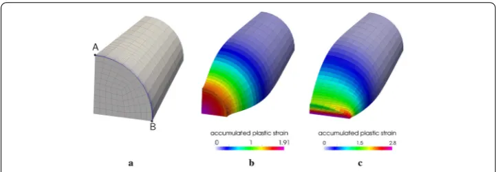
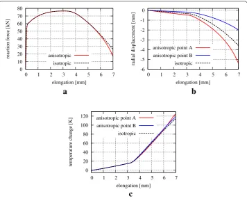
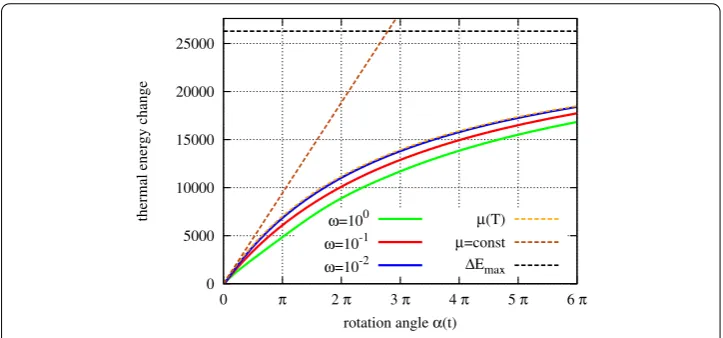
thermo-elasto-plastic frictional contact with finite deformations and finite strains is presented. A key feature is the reformulation of all involved inequality constraints, namely those of Hill’s orthotropic yield criterion as well as the normal and tangential contact constraints, in terms of non-smooth nonlinear complementarity functions. Using a consistent linearization, this system of equations can be solved with a non-smooth variant of Newton’s method. A quadrature point-wise decoupled plastic constraint enforcement and the use of so-called dual basis functions in the mortar contact formulation allow for a condensation of all additionally introduced variables, thus resulting in an efficient formulation that contains discrete displacement and temperature degrees of freedom only, while, at the same time, an exact constraint enforcement is assured. Numerical examples from thermo-plasticity, thermo-elastic frictional contact and thermo-elasto-plastic frictional contact demonstrate the wide range of applications covered by the presented method.

Keywords: Contact mechanics, Heat transfer, Frictional heating, Thermo-plasticity, Thermo-structure-interaction, Dual mortar methods

Introduction

In many engineering applications frictional contact and elasto-plastic material behavior come hand in hand. Just one class of typical well-known examples are metal forming and impact/crash analysis, where, at high strain rates, thermal effects need to be taken into account. The thermo-mechanical coupling appears in several forms: firstly and most obvi-ously, there is heat conduction across the contact interface. Secondly, the dissipation of frictional work leads to an additional heating at the contact interface. Thirdly, also plastic work within the structure is transformed to heat. Vice versa, the current temperature may influence the elastic and especially the plastic material response. All this necessitates robust and efficient solution algorithms for fully coupled thermo-elasto-plastic contact problems, which has been an active research topic over the past 25 years. Most

contribu-©The Author(s) 2018. This article is distributed under the terms of the Creative Commons Attribution 4.0 International License (http://creativecommons.org/licenses/by/4.0/), which permits unrestricted use, distribution, and reproduction in any medium, provided you give appropriate credit to the original author(s) and the source, provide a link to the Creative Commons license, and indicate if changes were made.

tions, however, focus either on thermo-plasticity or on thermo-mechanical contact, while resorting to relatively simple standard methods for the remaining problem parts.

Early implementations of thermo-elastic contact based on node-to-segment contact for-mulations in combination with a penalty constraint enforcement can be found in [1–7]. Within the last decade, more sophisticated variationally consistent contact discretizations based on the mortar method have been developed and applied to thermo-mechanical contact in [8–12]. In addition, those algorithms satisfy the contact constraints exactly (at least in a weak sense) by using either Lagrange multipliers or an augmented Lagrangian functional instead of a simple penalty approach. Due to an easier implementation and other benefits like symmetric operators, most of the cited works above employ some sort of partitioned solution scheme for solving the structural problem (at constant tempera-ture) and thermal problem (at constant displacement) sequentially. In thermo-plasticity, those partitioned schemes based on an isothermal split are only conditionally stable [13]. Only [4,6,11,12] employ monolithic solution schemes, which solve for displacements and temperatures simultaneously. Most developments of advanced computational methods in mechanical contact are restricted to elastic effects; coupled thermo-elasto-plastic contact can only be found in [5–7].

Numerical algorithms for finite deformation thermo-plasticity go back to the seminal work by Simo and Miehe [13], which is based on the isothermal radial return mapping algorithm presented in [14,15]. Both partitioned and monolithic solution approaches are discussed in [13]. Several extensions to this algorithm have been presented later, e.g. a monolithic formulation in principle axes [16] and a variant including temperature-dependent elastic material properties [17]. In a different line of work, a variational for-mulation of thermo-plasticity has been developed in [18], where the rate of plastic work converted to heat follows from a variational principle instead of being a (constant) mate-rial parameter as in [13]. A comparison to experimental results is presented in [19] to support this variational form. We point out that both approaches to determine the plastic dissipation, i.e. [13] and [18], are applicable within the algorithm for thermo-plasticity that will be derived in this manuscript. Besides the mentioned radial return mapping and variational formulations, a different numerical algorithm to isothermal plasticity at finite strains has been developed in [20]. Based on fundamental ideas from [21], the plastic deformation at every quadrature point is introduced as an additional primary variable and the plastic inequality constraints are reformulated as nonlinear complementarity functions. This allows for a constraint violation during the nonlinear solution procedure, i.e. in the pre-asymptotic range of Newton’s method, while ensuring their satisfaction at convergence. As usual in computational plasticity, the material constraints are enforced at each material point independently, such that the additional unknowns can be condensed directly at quadrature point level. It could be shown in [20] that due to this less restrictive formulation, a higher robustness can be achieved, which allows for larger time or load steps.

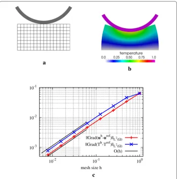
for the fully nonlinear thermo-mechanical contact formulation at the interface. Further-more, full compatibility of the algorithms for thermo-plasticity and thermo-mechanical contact is demonstrated. Concerning plasticity, an extension of [20] to coupled thermo-plasticity within a monolithic solution framework is presented. Similar to the isothermal case, the use of Gauss-point-wise decoupled plastic deformation allows for a condensa-tion of the addicondensa-tionally introduced plastic unknowns, where now also thermo-mechanical coupling terms have to be accounted for. The novel thermo-mechanical contact formu-lation represents a fully nonlinear extension of [12] including a consistent linearization with respect to both the displacement and temperature unknowns. Moreover, the use of dual Lagrange multipliers within a mortar contact formulation enables the trivial conden-sation of the discrete contact Lagrange multipliers such that the final linearized system to be solved consists of displacement and temperature degrees of freedom only. Our new thermo-mechanical contact formulation is applicable for both classical finite ele-ments based on Lagrange polynomial basis functions as well as isogeometric analysis using NURBS basis functions, for which an appropriate dual basis has recently been pro-posed in [22]. Owing to the variational basis of the mortar method, the thermo-mechanical contact patch test on non-matching discretizations is satisfied exactly and optimal con-vergence rates are achieved. Since this paper touches on various topics, and not every reader may be familiar with every single topic, we try to give a self-contained and rather detailed description of the different sub-problems and solution approaches. Even though this requires to some extent the repetition of methods developed elsewhere, we hope to thereby make the article and its novelties amenable to a broader audience.

The remainder of this paper is outlined as follows: “Thermo-plasticity in the bulk contin-uum” section contains the treatment of thermo-plasticity within the bulk structure from the underlying continuum mechanics to the final discrete system. “Thermo-mechanical contact” section then incorporates thermo-mechanical contact, again starting from a continuum description and closing with the linearized system that needs to be solved in each Newton iteration step. Finally, several challenging numerical examples in “Numer-ical results” section demonstrate the high accuracy and robustness that can be achieved for benchmark tests and more complex applications in elasto-plasticity, thermo-elastic contact and thermo-elasto-plastic contact.

Thermo-plasticity in the bulk continuum

sec-tion, those developments are used to construct a novel nonlinear solution procedure for thermo-plasticity using nonlinear complementarity functions. This can be seen as an extension of the authors’ previous work [20], where increased robustness in the isothermal case as compared to classical return mapping algorithms had been demonstrated in the isothermal case.

Continuum thermo-mechanics and thermo-plasticity

Let the closed set∈ 3be the reference configuration of a body andxthe current posi-tion of a material pointX∈at timetdefined by a bijective and orientation preserving mappingϕt(X)= x. Analogously, we define the current configurationt = ϕt(). The

surface∂is divided into the Dirichlet and Neumann boundary_mDand_mN, m∈ {u, T} for the displacementsuand the temperatureT, respectively. In the time interval of interest t∈[0, tE], the following initial boundary value problem (IBVP) must hold:

• Balance of mass:

˙

ρ0=0 in×(0, tE], (1)

• Balance of linear momentum:

DivP+bˆ0=ρ0u¨ in×(0, tE], (2)

• Balance of angular momentum:

PFT_=FPT _{in×(0, t}

E], (3)

• Balance of energy:

˙

E−P: ˙F+DivQ−R=0 in×(0, tE], (4)

• Clausius–Duhem inequality:

P: ˙F−E˙+Tη˙− 1

TQ·GradT ≥0 in×(0, tE], (5)

• Displacement Dirichlet boundary condition:

u=uˆ on_uD×(0, tE], (6)

• Displacement Neumann boundary condition:

PN=ˆ_{t0 on}N

u ×(0, tE], (7)

• Temperature Dirichlet boundary condition:

T =Tˆ on_TD×(0, tE], (8)

• Temperature Neumann boundary condition:

−QN=_Qˆ_{0 on}N

• Initial displacement:

u=u0 in×0, (10)

• Initial velocity:

˙

u=u˙0 in×0, (11)

• Initial temperature:

T =T0 in×0. (12)

In the IBVP above,ρ0denotes the mass density in reference configuration,F = Gradϕt

the deformation gradient,Pthe first Piola–Kirchhoff stress tensor,Ethe internal energy per unit undeformed volume,Ran energy source term per unit undeformed volume,ηthe entropy per unit undeformed volume,Qthe material heat flux, ˆuthe prescribed displace-ments, ˆt0the prescribed Piola–Kirchhoff tractions, ˆT the prescribed temperatures, and

ˆ

Q0the prescribed surface heat flux per area in reference configuration. If this heat flux

also depends on the temperature at the boundary (as in natural convection boundaries), Eq. (9) becomes a Robin-type boundary condition. Finally,u0, ˙u0andT0define the initial

displacements, velocities and temperature at time t = 0, respectively. First, we take a closer look at the last term in (5). From the fact that the absolute temperatureT is always positive, one can deduce that

Q·GradT ≤0. (13)

In spatial form, this can be assured by Duhamel’s law of heat conductionq = −κgradT for any symmetric positive definite conductivity tensorκ. Assuming isotropy, one obtains Fourier’s law of heat conductionq= −k0

J gradT with the scalar heat conductivityk0>0

and the Jacobian determinantJ =detF. The equivalent formulation in reference config-uration gives

Q= −k0C−1GradT, (14)

where C = FTFdenotes the right Cauchy–Green tensor. With (13) being assured, the Clausius–Duhem inequality (5) reduces to the Clausius–Planck inequality

Dint:=P: ˙F−E˙+Tη˙≥0. (15)

Next, we turn our attention to the formulation of elasto-plastic kinematics at finite defor-mations. As basic concept, we use a multiplicative split of the deformation gradient into an elastic partFe_{and a plastic partF}p_{as initially proposed in [28]:}

F=Fe_Fp_{. (16)}

Additionally, the entropy is decomposed additively into an elastic and a plastic part, i.e.η= ηe_+ηp_{. The plastic partη}p_{is associated with the entropy of the plastic configuration}

interested reader is referred to [13] for a more detailed discussion of this aspect. Moreover, we introduce an additional strain-like scalar internal variableαiassociated with isotropic hardening. Kinematic hardening may as well be included via an additional tensor valued internal variable, but for the sake of brevity it is not considered in this work; for an application of the plasticity algorithm presented later with kinematic hardening we refer to [20] and for a derivation of the associated continuum thermodynamics we refer to [18]. The internal energyEis defined as a function of the elastic state only, i.e.E =E(Fe,ηe). Introducing the Helmholtz free energy = E−T(η−ηp) one can reformulate the Clausius–Planck inequality and obtains

P: ˙F− ˙ −(η−ηp) ˙T +Tη˙p≥0. (17)

As usual in finite strain thermo-plasticity, the free energy is assumed to be decom-posed additively into an elastic energy contribution, an energy contribution due to work hardening and a thermal energy contribution:

=ρ0

ψe_(Fe_{, T)+ψ}p_(αi_{, T)+ψ}θ_{(T). (18)}

With the assumptions (16) and (18), the Clausius–Planck inequality (17) becomes

Dint=

P−ρ0∂ψ

e

∂Fe

∂Fe

∂F

: ˙F+

−(η−ηp)+ρ0∂ψ_∂

T

˙ T

+ρ0∂ψ

e

∂Fe

∂Fe

∂Fp : ˙F

p_+ρ

0∂ψ

p

∂αiα˙

i_+Tη˙p_≥0.

(19)

SinceF, ˙F,T and ˙Tmay take arbitrary values, we obtain the constitutive relations for the first and second Piola–Kirchhoff stressPandS, respectively

P=ρ0ψ

e

∂Fe

∂Fe

∂F =ρ0ψ

e

∂FeF

p−T_{, S=2ρ}

0Fp−1∂ψ

e

∂CeF

p−T_{, (20)}

as well as the elastic entropy

η−ηp_{= −ρ}

0∂ψ

∂T = −ρ0

∂(ψe_+ψp_+ψθ₎

∂T . (21)

The remaining terms in the dissipation inequality (19) read

Dint=ρ0∂ψ

e

∂Fe

∂Fe

∂Fp : ˙F

p_+ρ

0∂ψ

p

∂αi α˙

i_+Tη˙p_=:Dp_+ρ

0∂ψ

p

∂αiα˙ i

Dmech

+Tη˙p Dther

≥0, (22)

with the Mandel stress tensor = 2Ce∂ψe/∂Ce_{and the plastic velocity gradient} Lp =

˙

Fp_Fp−1_{. In case of elastic isotropy considered in the remainder of this paper, the Mandel}

stress tensorbecomes symmetric and the plastic velocity gradient Lp in (22) can be replaced by its symmetric partDp=sym( ˙Fp_Fp−1_{). Since the first two summands do not}

obtained by inserting (15), (21) and (22) into the energy balance (4). After some algebraic manipulations (see [13]), one obtains

CvT˙ = −DivQ+R+Dmech+T_∂∂

T(P: ˙F−Dmech)

Hep

, (23)

where we have introduced the elasto-plastic heatingHepand the specific heat capacity per unit undeformed volume

Cv= −ρ0T ∂ 2_ψ

∂T∂T. (24)

In many computational methods for finite deformation thermo-plasticity (e.g. [13,17, 29]), a simplified form of plastic heat generation is used based on a dissipation factorβ, sometimes also referred to as Taylor–Quinney factor. This simplification can also be taken here, i.e. the heat sources due to plasticity [(i.e.Dmech−T_∂∂TDmechin (23)] are replaced

by a fraction of the total plastic powerPpl=:Dp. Consequently, (23) becomes

CvT˙ = −DivQ+R+T∂

(P: ˙F)

∂T +βPpl. (25)

In metal plasticity, the dissipation factor is usually assumed to be in the range of β ∈ [0.85,1]. Within the later presented framework for finite deformation thermo-plasticity, both variants of the energy balance (23) and (25) can be implemented with similar computational effort.

Yield criterion and evolution of internal variables

In the previous section, we have developed the elastic and thermal constitutive relations of thermo-elasto-plasticity. We have, however, not yet decided on a specific plasticity model and flow rule to determine the evolution of the internal variablesFpandαi, with the only restriction being that the evolution equations must obey the dissipation inequality (22). In rate-independent elasto-plasticity, a yield function defines the set of admissible stress states. We will use an orthotropic yield function originally proposed by Hill [30]

fpl(,αi, T)=√:H:−

2 3

y0(T)+∂ψ

p_(αi_{, T)}

∂αi

= H−Ypl, (26)

which includes the well-known von Mises criterion as a special case of settingHto the deviatoric projection tensorPdev. For general orthotropic materials with the orthogonal axesni, i∈ {1,2,3}, the orthotropic tensorHis defined via the second order structural tensorsNi=ni⊗nias

H=α1N1⊗N1+α2N2⊗N2+α3N3⊗N3

+1/2(α₃−α₁−α₂)(N1⊗N2+N2⊗N1)

+1/2(α1−α2−α3)(N2⊗N3+N3⊗N2)

+1/2(α2−α3−α1)(N1⊗N3+N3⊗N1)

+α7(N1 N2+N2 N1)

+α8(N2 N3+N3 N2)

Therein, the tensor products of two symmetric second order tensors are defined as (A⊗

B)ijkl= AijBkland (A B)ijkl= 1/2(AikBjl+AjkBil). The coefficients are determined by

the relations of the normal yield stress yii in direction ofni, and the shear yield stress

yij, i=jin theni−nj-plane, respectively, with a reference yield stressy0:

α1=

2 3

y2₀ y2₁₁, α2=

2 3

y2₀ y2₂₂, α3=

2 3

y2₀ y2₃₃, α7=

1 3

y2₀ y2₁₂, α8=

1 3

y2₀ y2₂₃, α9=

1 3

y2₀ y2₁₃.

(28)

Since the tensor H includes a deviatoric projection, i.e. H = H : Pdev = Pdev : H, we may as well replace the Mandel stress in (26) by its deviatoric part and hence fpl(,αi, T) = fpl(dev,αi, T). Finally, the principle of maximum plastic dissipation provides the evolution equations

˙

Fp_Fp−1_=γ H:

H, (29)

˙ αi_=γ

2

3, (30)

subjected to the Karush–Kuhn–Tucker (KKT) type inequality constraints on the plastic multiplierγ

fpl ≤0, γ ≥0, fplγ =0, (31)

and the consistency condition

˙

fplγ =0. (32)

Assumptions on the used free energy

We want to briefly comment on some simplifying assumptions posed on the used free energy potential (18). Those simplifications are neither more nor less restrictive on the solution approach presented later than they are for classical radial return mapping algo-rithms for thermo-plasticity. Hence, they can often be found in the literature in a very similar way, for example in [13,17]. First, it is assumed that the elastic free energy can be decoupled into the following three summands:

ψe_(Fe_{, T)=M(J}e_{, T)+U(J}e_{)+W( ¯C}e_{). (33)}

As far as the isothermal response is concerned, this split implies a decoupled volumetric and isochoric elastic response, since Uonly depends on the elastic change of volume determined by the elastic Jacobian determinant Je _{= detF}e _{and Wonly depends on}

the volume preserving part of the elastic right Cauchy–Green tensor ¯Ce _{= J}e−2_/3_Ce_.

For the modeling of metallic materials, this is a widely used assumption that appears in the exact same way in almost every numerical algorithm for finite strain plasticity, see e.g. [14,15,24,31,32] and many more. The thermo-mechanical coupling is therefore restricted toM(Je, T). Following [13], we use

M(Je, T)= −3αT(T −T0)∂U

(Je)

which appears to be the logical extension of a linear small strain thermal expansion model to finite deformations. Therein,αT is the linear coefficient of thermal expansion

andT0a given reference temperature. In summary, the elastic potential (33) accounts

for thermal expansion, whereas the elastic material properties such as shear and bulk modulus do not depend on the temperature. A temperature dependent bulk modulus may easily be introduced combining UandMwithout any changes in the subsequent methods; the isochoric strain energy functionW, however, is assumed to be temperature independent. To this end, the deviatoric part of the Mandel stress devdoes not depend on the temperature, such that the only dependency on the temperature in the yield function (26) is throughYpl _=Ypl_(αi_{, T). The elastic heating term} ∂P: ˙F

∂T in (23) reduces to

∂P: ˙F ∂T =

∂2_M

∂T∂JeJ˙

e_{, (35)}

which is responsible for the so-called Gough–Joule effect. Finally, we choose the thermal energy potential as

ψθ_{(T)=Cv(T −T0)−Tlog}T T0

, (36)

and assume all other potentials in (18) to only depend (piece-wise) linearly on the temper-ature. As a consequence, the specific heat capacityCvdefined in (23) and further specified

in (24) reduces to a constant material parameter.

Weak form of the thermo-mechanical problem

To set the scene for the subsequent finite element discretization, we introduce the weak form of the thermo-mechanical problem. Therefore, appropriate solution and testing spacesU andVfor the displacement fielduand temperature fieldTare defined:

Uu=

uj∈H1(), j=1. . .3|uj=uˆj onDu(i)

, (37)

UT =T ∈H1() T =Tˆ onuT(i)

, (38)

Vu=

δuj∈H1(), j=1. . .3δuj=0 onuD(i)

, (39)

VT =

δT ∈H1() δT =0 on_TD(i). (40) The weak form of the coupled thermo-mechanical problem then consists of the balance of linear momentum (2) and heat conduction (23): Findu∈UuandT ∈UT, such that:

Gu =

δuρ0u¨d+

∇δu: (FS) d

−

δu·

ˆ

b0d−

N(i)

u

δu·ˆ_t0d=0 ∀δu∈Vu, (41)

GT =

δTρ0Cv

˙ Td−

∇δTQd

−

δT(R+Dmech+H

ep_{) d−}

N(i)

T

δTQˆ0d=0 ∀δT ∈VT. (42)

Additionally, the thermo-plastic constraints (29), (30) and (31) have to be satisfied locally, such that the thermo-mechanical coupling enters the structural equilibrium via the second Piola–Kirchhoff-stressS=S(u, T,Fp,αi). Vice versa, the thermal constitutive relation in (14) as well as the source termsDmechin (22) andHepin (23) introduce the coupling of

Spatial discretization of the thermo-mechanical continuum

The position, displacement and temperature field (as well as their variations) are approxi-mated in space using discrete nodal values (or control point values in case of isogeometric analysis (IGA))Xj,djandTjand ansatz functionsNj, viz.

Xh₌ n

j=1

NjXj, uh= n

j=1

Njdj, Th= n

j=1

NjTj. (43)

The ansatz functionsNjof nodejmay be either Lagrange polynomials for classical finite

elements or NURBS in the case of isogeometric analysis. The vectorsdandTcontain all displacement and temperature degrees of freedom in the approximation, respectively. As usual in finite element methods for plasticity, the plastic constraints (29), (30) and (31) are enforced locally at the quadrature points. The internal variablesFp_andαi_{are therefore}

assumed to be discontinuous and independent at every quadrature pointq, denoted asFpq

andαi_qin the following. Again, the vectorsFpandαirepresent the union of all discrete values at the quadrature points.

Remark 1 All algorithms presented later are directly applicable to both finite elements and isogeometric analysis, such that no further distinction will be made in the following. For the sake of brevity, no introduction to isogeometric analysis will be given here, since there has been an overwhelming amount of publications on IGA in the past decade, including the monograph [25]. For details on the application of the dual mortar method to isothermal isogeometric contact mechanics, we refer to our recent work [22].

The spatial discretization (43) can now be inserted into the weak form of the balance of linear momentum in (41), while still neglecting the contact contribution for now. The discrete algebraic force equilibrium becomes:

δda

⎡ ⎢ ⎢ ⎢ ⎢ ⎣

hNaρ0Nbd

¨ db

finert

u =Mud¨ +

h∇Na: (FS) d

fint

u (d,T,Fp,αi)

−

hNa

ˆ

b0d+

Nh

u

Naˆ_t0d

fext

u

⎤ ⎥ ⎥ ⎥ ⎥

⎦=0, (44)

or in short

Mu_d¨_+fint

u (d,T,Fp,αi)−fuext=0, (45)

The same discretization can be applied to the weak form of the heat conduction equation, which gives

δTa

⎡ ⎢ ⎢ ⎢ ⎢ ⎣

hNaρ0CvNbd

˙

Tb

finert

T =MTT˙ +

h∇Na(k0C

−1_)∇N

bdTb

fint

T (d,T)

−

hNaRd+

Nh

T

NaQˆ0d

fext

T

−

hNa(Dmech+H

ep_{) d}

fdiss

T (d,T,Fp,αi)

⎤ ⎥ ⎥ ⎥ ⎥ ⎥

⎦=

0, (46)

or in short

MT_T˙_+fint

T (d,T)−fText−fTdiss(d,T,Fp,αi)=0. (47)

Similar to the structural equilibrium above, the mass matrixMT determining the heat capacity is constant and the internal load vectorf_Tintdepends linearly on the temperature and nonlinearly on the displacement via Fourier’s law of heat conduction in the finite deformation realm, see (14). The discrete mechanical dissipation vector f_Tdissdepends nonlinearly on the displacement and the plastic deformation at every quadrature point according to (22) and (23). Finally, for both the structural and the thermal problem, the external load vectorsf_{ext_u,T}are assumed to be independent of the displacement and temperature field for the sake of simplicity.

Time discretization

To discretize the semi-discrete equilibrium (45) and (47) in time, we apply generalized-α schemes, which are of second-order accuracy, and can be formulated with the spectral radius in the high frequency limitρ∞ as sole parameter. For structural problems, this method has been presented in [26]. The approximation of discrete velocitiesvand accel-erationsais based on the Newmark-scheme, viz.

n+1_v= γu

βut

(n+1d−nd)−γu−βu βu

n_v− γu−2βu

2βu

tna,

n+1_a= γu

βut2

(n+1d−nd)− 1 βut

n_v−1−2βu

2βu n_a,

(48)

wheretdenotes the time step size of the interval [n_t,n+1_{t]. The left superscript signifies}

the approximation at the discrete timen_tandn+1_{t, respectively. The discrete equilibrium}

(45) is then evaluated at a generalized mid-point by introducing the parametersαu,f and

αu,m:

ru =Mun+1−αu,m_a+n+1−αu,ffint

u −n+1−αu,ffextu =0. (49)

The discrete forces (and accelerations) at the mid-points are eventually interpolated by the forces (and accelerations) at the end of each time step, e.g.n+1−αu,ffint

αu,fnfintu . In [26], an optimal set of parameters is derived in terms of the spectral radius in

the high frequency limitρu,∞as

αu,m=

2ρu,∞−1

ρu,∞+1

, α_u,f = ρu,∞ ρu,∞+1

, (50)

βu =

1

4(1−αu,m+αu,f)

2_{, γ}

u=

1

2 −αu,m+αu,f. (51) The generalized-αmethod has been extended to systems of first order in time in [27], which will be used for the temporal discretization of the thermal evolution (47). Similar to (48), the temperature rate is approximated by

n+1_˙

T= 1 γTt

(n+1T−nT)−1−γT γT

n_˙

T. (52)

Again, the discrete equilibrium (47) is evaluated at a generalized mid-point defined by αT,mandαT,f:

rT =Mn+αT,m_˙

T+n+αT,f_fint

T −

n+αT,f_fext

T −

n+αT,f_fdiss

T =0, (53)

where the values at the mid-points are again obtained by an appropriate linear combination of the end-point values. An optimal choice of the parameters has been derived in [27] in terms of the spectral radius in the high frequency limitρT,∞as

αT,f =

1

ρT,∞+1, αT,m= 1 2

3−ρT,∞

ρT,∞+1, γT = 1

2+αT,m−αT,f. (54)

Finally, we need a discrete time integration of the evolution equations for the internal plastic variables in (29) and (30). Here, we follow standard techniques in finite strain plas-ticity, see e.g. [24], namely an exponential map time integration for the plastic deformation gradient and a backward-Euler scheme for the other internal variables, viz.

n+1

Fpq=exp

γq

H:n+1q

n+1

qH

n

Fpq, n+1

αi

q=

2 3γq+

n

αi

q, (55)

where the plastic multiplier incrementγqmust be determined such that the Karush–

Kuhn–Tucker conditions (31) are fulfilled at timen+1t. The advantage of the exponential map here is that it preserves the plastic incompressibility in the time-discrete setting. This means that if the plastic constitutive equations are such that plastic deformation does not result in a change of volume (i.e. det[Fp]≡1∀t), the argument of the exponential function is traceless, and hence, we also get det[nFp]≡1∀nin the time-discrete setting.

Solution algorithm using nonlinear complementarity functions

A similar approach to the one described in the following has been developed for small strain von Mises plasticity in [21] and extended to finite deformation anisotropic Hill-type plasticity in [20]. We therefore introduce the incremental plastic flow Dpq =

γq H: n+1

q

n+1

qHat each quadrature pointqas an additional primary variable and can express

the evolution equations (55) solely in terms of this incremental plastic deformation, viz.

n+1

Fpq=exp

Dpq

n

Fpq, (56)

n+1_αi

q=nαiq+max

0,

2 3

_q

HDpq:H:q

_H:q2

. (57)

Then, we introduce a trial value for the Mandel stress

tr

q =dev+cplH+:Dpq, cpl>0, (58)

where the pseudo-inverseH+ofHhas been used. The plastic inequality constraint is then equivalent to finding the root of the complementarity function

Cpl

q(d,T,Dpq)=

devq−min

1, Y

pl q

tr

qH

tr

q

maxYqpl,qtrH

, (59)

at each quadrature pointq. Here, the temperature only enters via the temperature depen-dent yield stressYqpl; the (deviatoric part of the) Mandel stress is temperature independent

due to the assumed restrictions on the used free energy (33). Temperature dependent elas-tic material properties (and hence a temperature dependency of dev) may be included, but would further complicate the derivative∂Cqpl/∂Tneeded later and are therefore omitted

here for the time being for the sake of simplicity.

The set of nonlinear equations that needs to be solved in every time step of a thermo-elasto-plastic problem without contact consists of the balance of linear momentum (49) and the heat conduction (53) complemented with the NCP function (59) at every quadra-ture point. Since this system is semi-smooth, variants of Newton’s method can be applied resulting in the linearized system

∂ru

∂dd+ ∂ru

∂TT+ ∂ru

∂Dp(D

p_{)= −ru, (60)}

∂rT

∂dd+ ∂rT

∂TT+ ∂rT

∂Dp(D

p_{)= −rT, (61)}

∂Cpl q

∂d d+ ∂Cpl

q

∂T T+ ∂Cpl

q

∂Dpq

(Dpq)= −Cplq, ∀q∈G, (62)

where the setGcontains all potentially plastifying quadrature points. For brevity, the detailed structure of the involved linearizations are omitted here, since they have either already been presented for the isothermal case in [20] or follow from similar calculations as given therein. The system (60)–(62), however, is of significantly increased size compared to the original number of displacement and temperature degrees of freedom, since at every quadrature point, assuming a symmetric and traceless incremental plastic flow Dpq,

Dplq from (60)–(62) is the fact that (62) only contains the discrete plastic increment of

one quadrature point as well as the displacement and temperature degrees of freedom belonging to the element containing this quadrature point. Hence, the linearized plastic NCP function (62) can be solved directly for the increments(Dplq) at the level of

quadrature points, yielding

(Dplq)= −

∂Cpl

q

∂Dpq

−1

Cpl

q + ∂C

pl q

∂d d+ ∂Cpl

q

∂T T

. (63)

This condensation can in turn be inserted into (60) and (61) and results in modified linearizations with respect to the displacements and temperatures in those equations, which will be indicated by a tilde ˜(·). Specifically, one obtains

˜

K{u,T}u= ∂r{u,T}

∂d −

q∈G ⎡ ⎣

∂r{u,T}

∂Dpq

∂Cpl q

∂Dpq

−1

∂Cpl q

∂d

⎤

⎦, (64)

˜

K{u,T}T = ∂r{u,T}

∂T −

q∈G ⎡ ⎣

∂r{u,T}

∂Dpq

∂Cpl q

∂Dpq

−1

∂Cpl q

∂T

⎤

⎦, (65)

˜

r{u,T}=r{u,T}−

q∈G ⎡ ⎣

∂r{u,T}

∂Dpq

∂Cpl q

∂Dpq

−1

Cpl q

⎤

⎦. (66)

After having solved for the displacement and temperature incrementsdandTin the current Newton iteration, the condensation equation in (63) can be used to recover the increments of the plastic deformation(Dpq) at each quadrature pointq. The matrices

Thermo-mechanical contact

Having dealt with the thermo-mechanical coupling within the bulk structure, we turn our focus to thermo-mechanical contact problems. First, the continuum mechanical description is recalled in “Problem setup” section, which, in more detail, can also be found e.g. in [42,43]. Next, a weak form extending the small strain formulation presented in [12] is derived in “Weak form of the thermo-mechanical contact problem” section. Finally, we present the new mortar finite element formulation for finite deformation mechanical contact problems in “Mortar finite element discretization of thermo-mechanical contact” section.

Problem setup

We consider a two body finite deformation thermo-mechanical contact problem in three spatial dimensions. Let the closed sets(i)⊂ 3, i=1,2 be the reference configuration of the two bodies. Both bodies are governed by the IBVP described in “Thermo-plasticity in the bulk continuum”, enhanced with the constraints of frictional contact at the potential contact boundaryC(i). The boundary∂(i)is hence decomposed into three subsets such that ∂(i) ₌ D(i)

u ∪Nu(i)∪C(i) = _TD(i)∪_TN(i)∪C(i) and ∅ = uD(i)∩Nu(i) =

D(i)

u ∩C(i) = uN(i)∩C(i) = _TD(i)∩_TN(i) = D_T(i)∩C(i) = N_T(i)∩C(i). Since

the focus is on finite deformations, the geometrical contact constraints such as the non-penetration condition have to be satisfied in the current configuration, i.e. they have to be enforced between the current potential contact surfacesγC(i) = ϕt(C(i)). Applying

standard nomenclature in contact mechanics, we will refer toγC(1)as theslavesurface, and toγC(2)as themastersurface. For a pointx(1)on the slave surface (in spatial configuration), one can find an associated point ˆx(2)on the master surface by projectingx(1) along its current outward normal vectorn. With those points at hand, the normal gapgnand the

relative tangential velocity are defined by

gn= −n

x(1)_−xˆ(2) _{, (67)}

vτ =(1−n⊗n)

˙

x(1)_−x˙ˆ(2) _{, (68)}

where ˙x(1)_{and ˙ˆx}(2)_{denote the material velocities ofx}(1)_{and ˆx}(2)_{, respectively. The contact}

tractiontcat the interface is decomposed in the same way to obtain the normal contact pressurepnand the tangential contact tractiontτ, viz.

pn= n t(1)c , tτ =(1−n⊗n)tc(1). (69)

The mechanical contact constraints can then be formulated in normal direction via the Hertz–Signorini–Moreau condition and in tangential direction by Coulomb’s law of fric-tion on the slave contact surface:

gn ≥ 0, pn≤0, pngn=0 onγc(1), (70)

ffr := tτ −μ(θc)|pn| ≤0, vτ+βtτ =0, β≥0, ffrβ=0 onγc(1), (71)

together with the consistency conditions in normal and tangential direction

˙

The master side contact traction follows directly from the balance of linear momentum

t(2)

c = −tc(1). Since we are interested in a fully coupled thermo-mechanical contact

prob-lem, we allow for a temperature dependent friction coefficientμ(θc) depending on the

maximal temperature of the contact surfacesθc = max[T(1)(x(1)), T(2)(ˆx(2))]. Following

[42], an exemplary temperature dependency of the friction coefficient is introduced as

μ(θc)=μ0

(θc−Td)2

(T_d−T0)2

(73)

via a reference coefficient of frictionμ0at the reference temperatureT0and a damage

temperatureTd >T0. The apparent coefficient of friction decreases monotonically from

μ0atT0to zero atTd. The damage temperatureTd is usually chosen to be the lower

melting temperature of the two contacting materials, since at this point, friction is no longer dominated by solid shearing but rather by viscous effects in a thin film of molten material.

Next, the local energy balance at the contact interface is investigated. For simplicity, we assume that the interface has no heat capacity by itself, i.e. the specific internal energyec

is zero at all times. Written in rate form one obtains

0=e˙c=tτvτ+qc(1)+q(2)c , (74)

whereqc(i)=q(i)n(i)denotes the spatial (Cauchy) heat flux at the two contact surfaces. A

possible choice of the heat fluxes at the contact interface is given in [2,42] as

q(_ci)=γ(i)(T(i)−Tc), γ(i)=γ¯(i)pn. (75)

Here, the heat transfer parameterγ(i)has been chosen as a simple linear function of the normal contact pressure. Yet, any nonlinear relation may be employed as long as a zero contact pressure (i.e. no contact) relates to a zero heat flux over the contact interface. Using (74) and (75) and eliminating the contact surface temperatureTcfrom the system,

the spatial heat fluxes can be stated as

q(1)_c =βcpn[T]−δctτvτ, (76)

q(2)_c = −q_c(1)−t_τv_τ, (77)

with the temperature jump over the contact interface [T]= (T(1)−T(2)) as well as the coefficientsβc= γ¯

(1)_γ¯(2)

¯

γ(1)_+γ¯(2) andδc=

¯

γ(1)

¯

γ(1)_+γ¯(2) defined according to [2,12].

Remark 4 The parametersβcandδcalso have a direct physical interpretation: The

prod-uctβcpn in (76) and (77) determines the heat flux across the contact interface due to

the temperature jump, i.e. it describes the contact heat conductance. In the presented description, which follows [2,42], the heat flux is a linear function of the contact pressure. However, more involved nonlinear relations can be found in the literature. For instance, [43] distinguishes three sources of heat conduction across rough surfaces: conduction through contacting asperities, heat conduction in enclosed gas and radiation. In the for-mulation presented later, nonlinear models for heat conduction could be employed simply by replacing the productβcpnwith a nonlinear relation ¯βc(pn) or, when formulated using

the later defined Lagrange multipliers (representing the negative contact traction), by replacingβcλcnwith−β¯c(−λcn) in (95).

The parameterδcdetermines how frictional heat is distributed to the two bodies. In the

limit casesδc=0 orδc=1 the entire frictional heat is added to the master or slave side,

respectively.

Weak form of the thermo-mechanical contact problem

To prepare the subsequent mortar finite element discretization of the thermo-mechanical contact problem, the weak form of the thermo-structure-interaction problem in (41) and (42) is extended to account for the effects of frictional contact. Therefore, two Lagrange multiplier fields are introduced at the contact interface; a vector-valued Lagrange multi-plier to enforce the mechanical contact constraints (70) and (71), which can be identified as the negative slave side contact tractionλc= −tc(1), and a scalar Lagrange multiplier to

enforce the heat flux constraints over the contact interface in (76) and (77), which will be chosen as the slave side heat fluxλθ =qc(1). The contact Lagrange multiplier is taken from

the convex set

M(λ) :=!μ∈Mμ,v_γC(1) ≤ μλc_n,vτ_γC(1),v∈Wwithvn≤0

"

, (78)

whereWdenotes the trace space ofUuonγC(1),Mits dual space, and·,·_γC(1)denotes the scalar or vector-valued duality pairing between W andMonγC(1)_{. The contact}

Lagrange multiplier is decomposed into a normal partλc

nand a tangential partλcτ

analo-gously to the contact traction in (69). The thermal Lagrange multiplier is chosen from the (scalar valued) dual spaceMonγC(1). The complete weak form of the coupled thermo-mechanical contact problem then reads : Find u(i) ∈ U(_ui), T(i) ∈ U_T(i), λc ∈ M(λc), λθ_{∈M, such that:}

2

i=1

G_u(i)+

γC(1)

δu(1)_−δu(2)_◦P

t

·λc_dγ

Gc u

=0 ∀δu(i)∈V(_ui), (79)

2

i=1

G_T(i)−

γC(1)

δT(1)−δT(2)◦Pt

λθdγ +

γC(1)

δT(2)◦Pt

λc_·v

τdγ

G_Tc

=0

∀δT(i)∈V_T(i), (80)

Hu=

γC(1)

δλc

n−λcn

gndγ −

γC(1)

δλc

HT =

γC(1)δλ

θ_λθ_{dγ +}

γC(1)δλ

θ_β

cλcn

T(1)−

T(2)◦Pt

dγ

+

γC(1)δλ

θ_δ

cλcvτdγ =0 ∀δλθ∈M. (82)

Therein, all integrals over the contact surfaces of the two bodies have been transformed into pure slave side integrals by using a suitable mappingPt :γC(1)→γC(2)at timet.

Mortar finite element discretization of thermo-mechanical contact

The discrete interpolation of displacements and temperatures at the contact interface follows directly from (43) by restricting the ansatz functions to the element boundary. In the present notation, we will not explicitly distinguish between the ansatz functions in the continuum and at the boundary. Instead, the context will provide the necessary information, i.e. if the quantities are integrated over a volume, the ansatz functions refer to (43) and if integration is performed on the contact surface only the trace space restriction of the ansatz functions are evaluated.

Both the contact Lagrange multiplier λc and the thermal Lagrange multiplierλθ are interpolated by dual basis functionsjand discrete nodal valuesλcj andλθj, respectively:

λc,h₌ j∈S

jλcj, λθ,h=

j∈S

jλθj, (83)

where the setScontains all nodes on the slave contact surface. The dual basis functions are constructed such that they fulfill a biorthogonality condition [44]

γC(1)hi

Njdγ =δij

γC(1)h

Njdγ, (84)

where δij denotes the Kronecker symbol, i.e.δij = 1 ifi = jandδij = 0 otherwise. In

practice, the easiest way to define those dual basis functions is via an element-wise linear combination of the standard ansatz functionsNi, see e.g. [44], which at least ensures a

partition of unity property. For details on their construction, linearization and application to contact mechanics with small and large deformations including friction, the reader is referred, for instance, to [45–50], and for a first application to thermo-elastic contact to [12]. With the discretization of the displacement and temperature field (43) and the discrete Lagrange multipliers (83), we can now approach the contact related parts in (79)–(82) and discretize them adequately in space and time.

First, we consider the contact contributionG_ucin the weak balance of linear momentum in (79). Inserting the discretization yields

G_uhc=

j∈S

k∈S δd(1)_k

γC(1)hjN

(1)

k dγλcj −

j∈S

l∈M δd(2)_l

γC(1)hj(N

(2)

l ◦Pth) dγλcj,

(85)

where the setMcontains all nodes of the master contact surface andP_thdenotes a discrete version of the projection Pt introduced in (79). The first integral in (85) constitutes a

square coupling matrixDu, which obviously becomes diagonal when using the dual basis

those matrix blocks and by re-arranging the vector of displacement degrees of freedom d=[dN,dM,dS]T, wheredSanddMcontains all degrees of freedom on the slave and master contact surface, respectively, andd_N all other nodal displacements, the discrete contact force is obtained as

fc

u=[0,−Mu(d),Du(d)]Tλc. (86)

The displacement dependency of the coupling matrices is a consequence of the projection P_thand the integration, which has to be performed on the current configuration of the contact surfaceγC(1)h_{. Next, this contact force has to be incorporated in the time-discrete}

balance of linear momentum (49). This is done in a fully implicit way, so that the space and time discrete equilibrium (49) is complemented with a contact contribution

rc

u =Mun+1−αu,ma+n+1−αu,ffintu −n+1−αu,ffextu +n+1fcu=0. (87)

Remark 5 By choosing a fully implicit time discretization of the contact forces instead of some linear combination ofn+1fc_uandnfc_u, we guarantee that the contact work in one time stepWc = (n+1d−nd)Tn+1fc_ubecomes negative (i.e. dissipative) for nodes that come into contact and zero for nodes leaving the active contact set. Following an idea in [51] the dissipated energy can be re-introduced into the system via a velocity update procedure. If, however, the contact force were discretized by a linear combination of two time steps, nodes leaving the active contact set would introduce energy to the discrete system, which one might not be able to compensate via the velocity update procedure.

The next contact contribution to be discretized is the contribution to the heat conduc-tion equaconduc-tion (80). A strict applicaconduc-tion of the discretizaconduc-tion (43) and (83) would give

G_Thc=

j∈S

k∈S δT_k(1)

γC(1)hjN

(1)

k dγλθj

−

j∈S

l∈M δT_l(2)

γC(1)hj

(N_l(2)◦P_th) dγλθ_j

+

j∈S

l∈M

λc

τj

γC(1)hj(1−n⊗n)

×

k∈S

N_k(1)v(1)_k −

m∈M

N_m(2)vˆ(2)_m

◦Ph_t

(N_l(2)◦P_th) dγ δT(2)_l . (88)

The first and second part therein stem from the heat conduction over the contact interface and result in the similar coupling matricesDTandMTalready used in the structural

the computational cost by appropriate lumping techniques in the discrete representation of (80) and (82). Therefore, we introduce a frame indifferent weighted nodal tangential velocity ˜v_τjderived from a (discrete) time derivative of the mortar matricesDuandMuas

˜

v_τj= −(1−n⊗n)

k∈S ˙ Djkx(1)_k −

l∈M ˙ Mjlx(2)_l

, (89)

see [50,52,53] for details. The last summand in (88) is then replaced by

j∈S

l∈M δT(2)_l

γC(1)hk(N

(2)

l ◦Pth) dγ

˜ v_τk·λc_τk

#

γC(1)hkdγ

. (90)

From a physical point of view, this means that we do not interpolate the velocities and the contact Lagrange multiplier but only the scalar product v˜τj·λ

c τj #

γC(1)hjdγ =D c

mech,j, which

represents the frictional dissipation power at the slave node. Numerically, (90) implies a lumping of the triple integrals in (88), thus resulting in an integral over the product of two ansatz functions only. The contact contribution to the discrete thermal equilibrium (53) is again interpolated at the mid-pointn+αT,ffc

T =αT,fn+1fcT+(1−αT,f)nfcT, such that rc

T =M

n+αT,m_˙

T+n+αT,ff_Tint−n+αT,f_fext

T −

n+αT,f_fdiss

T +n+αT,ffcT =0, (91)

with

n_fc

T =

0,−MT(nd),DT(nd)

Tn_λθ_+0,M

T(nd),0

Tn_Dc

mech, (92)

where the vectorDc_mechcontains all entries of the contact dissipation power at all nodes Dc

mech,j.

Still, the interface constraintsHuandHTin (81) and (82) need to be discretized. Owing

to the biorthogonality of the dual basis functions for the Lagrange multiplier (84), it is well-known that the discretization of the variational inequality (81) yields decoupled constraints for the nodes [45,48]. The discrete normal contact constraint becomes

˜ gj:=

γC(1)hjgn,hdγ ≥0, λnj≥0, λnj

˜

gj=0, (93)

where ˜gjis called weighted gap at nodej. Analogously, the frictional constraint becomes

f_jfr := λ_τj −μ(θcj)|λnj| ≤0, v˜τj+βλτj=0, βj ≥0, f_jfrβj=0. (94)

In the fully coupled thermo-mechanical contact problem, the coefficient of friction depends on the temperatures at the two sides of the contact interface, e.g. via (73). In the discrete setting we determine the maximal contact interface temperatureθcj =

Finally, a discrete representation of the thermal interface condition (82) is required. At this point, we again deviate from a strict application of the discretization, as we already did in (90), and end up with the following discrete representation of (82):

δλθ ·Dθ =H_Th =

j∈S δλθj

γC(1)h

Njdγλθj

+

j∈S

δλθjβcλcnj

k∈S

γC(1)hj

N_k(1)dγT_k

−

l∈M

γC(1)hj

(N_l(2)◦P_th) dγTl

+

j∈S

l∈M

δλθj(˜vτj·λτj)

γC(1)hδcj

(N_l(2)◦P_th) dγ =0 ∀δλθ_j. (95)

Thanks to the lumping procedure, especially for the first integral, the thermal interface condition decouples for the contact nodes j, i.e. we can setλθ to zero for all inactive contact nodes. For the contact interface constraints, this decoupling can be achieved in a consistent manner using dual shape functions, such that only local, decoupled constraints have to be solved instead of an inequality constraint coupling all interface nodes. To keep up this advantage in the coupled thermo-mechanical contact problem, the presented lumping is required, see [12] for a more detailed discussion. We want to emphasize that for standard thermo-mechanical mortar methods, e.g. [11], a similar simplification is made implicitly by using a node-wise decoupled active set strategy, although strictly speaking the variational inequality does not not allow for such a decoupled treatment in that case [54,55].

Solution algorithm using nonlinear complementarity functions

The discrete system derived in the previous section still includes discrete inequality con-straints for normal contact (93) and Coulomb friction (94) at all slave nodesS. As com-monly used in isothermal dual mortar methods, the contact constraints are reformulated as nonlinear complementarity (NCP) functions, which then pose non-smooth equality constraints to the system, see e.g. [45,47,54]. A first application to small-strain thermo-elastic contact problems was presented in [12]. However, a fixed-point solution approach for the thermal interface conditions was used, thus sacrificing a quadratic rate of con-vergence. In this work, the concept of NCP functions will only be briefly reviewed by highlighting the additional complexity resulting from thermo-mechanical coupling. At each slave node, we define the trial values

λc,tr

nj =λcnj−cng˜j, cn>0, (96)

λc,tr

τj =λcτj+cttvj˜, ct>0. (97)