R E S E A R C H A R T I C L E
Open Access
Effect of the separated approximation of
input data in the accuracy of the resulting
PGD solution
Sergio Zlotnik
1*, Pedro Díez
1, David Gonzalez
2, Elías Cueto
2and Antonio Huerta
1*Correspondence:
[email protected] 1Laboratori de Calcul Numeric (LaCaN), E.T.S. de Ingenieros de Caminos, Canales y Puertos, Universitat Politecnica de Catalunya, Jordi Girona 1, 08034 Barcelona, Spain
Full list of author information is available at the end of the article
Abstract
The proper generalized decomposition (PGD) requires separability of the input data (e.g. physical properties, source term, boundary conditions, initial state). In many cases the input data is not expressed in a separated form and it has to be replaced by some separable approximation. These approximations constitute a new error source that, in some cases, may dominate the standard ones (discretization, truncation…) and control the final accuracy of the PGD solution. In this work the relation between errors in the separated input data and the errors induced in the PGD solution is discussed. Error estimators proposed for homogenized problems and oscillation terms are adapted to asses the behaviour of the PGD errors resulting from approximated input data. The PGD is stable with respect to error in the separated data, with no critical amplification of the perturbations. Interestingly, we identified a high sensitiveness of the resulting accuracy on the selection of the sampling grid used to compute the separated data. The separation has to be performed on the basis of values sampled at integration points: sampling at the nodes defining the functional interpolation results in an important loss of accuracy. For the case of a Poisson problem separated in the spatial coordinates (a complex diffusivity function requires a separable approximation), the final PGD error is linear with the truncation error of the separated data. This relation is used to estimate the number of terms required in the separated data, that has to be in good agreement with the truncation error accepted in the PGD truncation (tolerance for the stoping criteria in the enrichment procedure). A sensible choice for the prescribed accuracy of the PGD solution has to be kept within the limits set by the errors in the separated input data.
Keywords: Proper generalized decomposition, Error assessment, Separable functions
Background
The Proper Generalized Decomposition (PGD) [1,2] is ana priorireduced basis technique designed to deal efficiently with highly-dimensional Boundary Value Problems (BVP). Dif-ferently from other discretisation techniques such as Finite Elements or Finite Differences, PGD avoids the exponential growth of the number of degrees of freedom with the number of dimensions. This is achieved by means of a separated representation of the solution. A
separable function f with rankq, separated onndimensions has the form,
©2015 Zlotnik et al. This article is distributed under the terms of the Creative Commons Attribution 4.0 International License (http:// creativecommons.org/licenses/by/4.0/), which permits unrestricted use, distribution, and reproduction in any medium, provided you give appropriate credit to the original author(s) and the source, provide a link to the Creative Commons license, and indicate if changes were made.
f(x1, x2,. . ., xn)= q
m=1
Fxm1(x1)Fxm2(x2). . .F
m xn(xn)=
q
m=1
n
p=1
Fxmp(xp). (1)
The key benefit of the use of a separable solution is to transform the multidimen-sional integrals arising in the weak form of the problem into products of single (or lower) dimensional integrals. This can be done as the integral of a separated function
s(x, y, z)=f(x)g(y)h(z) can be written as,
x y z
s(x, y, z)dx dy dx=
x
f(x)dx
y
g(y)dy
z
h(z)dx. (2) The evaluation of 3 one-dimensional integrals of the right hand side requires smaller computational effort compared with its left hand side. The key idea is to apply the same separation strategy to the integrals arising in the weak form. A more detailed explanation of this procedure is given in Sect. “Problem statement and PGD solution for separated space dimensions”. However, as indicated in Eq. (2), not only the solution of the problem but all the functions involved in the operators must be separable. The typical functions present are material properties (thermal diffusivity, viscosity, density, etc.), initial or boundary conditions, and source terms, among others. In practice these functions usually do not admit an exact separable representation. The example used in this work consists in a Pois-son problem including a non separable diffusivity function. Diffusivity could be defined by empirical laws or a fitting function of laboratory measurements; its expression then will be hardly separable. In those cases, in order to apply PGD it is usual to replace the non-separable function by a non-separableapproximationto it. Section “Separation of the input data” presents one procedure to obtain separable approximations of known functions based on singular value decomposition.
Section “Results” shows results of a Poisson problem including the following non-separable diffusivity function:
k(x, y)=sin0.5(x+y)2+2. (3) To apply PGD,kit is replaced by an approximation with the form
k(x, y)≈ksep(x, y)= nk
l=1
Glx(x)Gly(y). (4) The separation procedures usually work with discrete (mesh based) versions of the func-tion. Therefore, this separation introduces two new sources of errors that are not present in the traditional Finite Element approach. First, a truncation error is introduced due to the finite number of terms (nk) used to describeksep. Second, an interpolation error in the spatial representation of the functionsGxl(x) andGly(y) similar to the usual FE error is also included. The goal of this work is to study the relation between these errors and the accuracy of the PGD solution. This relation can be useful to determine the number of termsnk required to achieve a certain accuracy by PGD. Moreover, this relation can also be used as stopping criteria for the PGD enrichment process, because the PGD solution will be at most as accurate asksep.
Motivation examples
faced PGD convergence problems in some more complex examples. Two of these prob-lems are briefly described next.
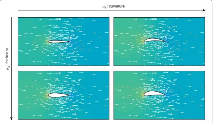
The first example was found while solving a BVP with parameterized geometry. In that case the shape of the domain, or the location of internal interfaces, depend on a set of parameters. Figure 1shows a parameter dependant geometry for an airfoil and the objective is to find the air flow around it. The method applied was proposed in [3] and later extended in [4]. It is based on the idea of having a reference domainT and a mapping function that relates all possible geometries to the reference domain. In practice, this mapping introduces some Jacobians depending on the parameters to the equation and, therefore, the dependence of the problem on the geometrical parameters becomes explicit. For example, the usual bilinear form for a Poisson problem reads
a(u, v)=
(µ)∇
u·(k∇v)d=
T ∇xˆu·
k|J(µ)|J(µ)−TJ(µ)−1
D(µ)
∇xˆvdxˆ
where ˆx are the reference coordinates. The matrixD(µ), including all the Jacobians, accounts for the geometrical parameterization. The analytical expression of D(µ) is known, but it is not separable. An approximation to it is therefore utilized in practice. The discretization used in the separation ofDwas found of to be of key importance in order keep the convergence of PGD. The truncation errors are also relevant and ultimately may control the final convergence that PGD could attain.
A second example arises in a scheme proposed in [5] for the real-time integration of solid dynamics equations. The scheme combines Proper Orthogonal Decomposition (POD) and PGD approaches and it is based upon a parametric formulation depending on the initial conditions. It implements a direct time integrator that can be seen as a sort of black-box: it that takes the resulting displacement field of the current time step as input and (via POD) provides the result for the subsequent time step. In order to reduce the high dimensionality produced by the large amount of parameters describing the initial
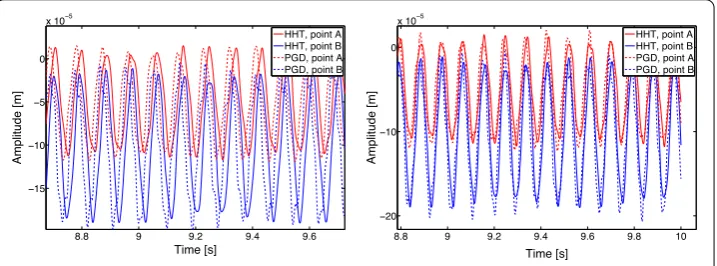
Fig. 2 Motivation example: real-time integration of solid dynamics. The initial conditions of the problem are separated.Leftandright panelshow the solution of the problem when the input data is separated with 3 and 8 terms, respectively. In the former case there is an error in the amplitude and also in the phase, while in the later the error is only in the amplitude and the phase is corrected
displacement field a reduced basis is obtained using PGD. This step introduces again a truncation error that will affect the final convergence of the proposed scheme. Figure2 shows two results with 3 and 8 terms in the approximation of the input data (initial conditions). Note that the solution including only 3 terms presents phase errors that disappear for the 8 terms solution.
A priori estimates for FE
Different sources of errors are present in the solution provided by PGD (see for example [6–8]. Ifuis the analytical solution of the BVP anduH,M is the solution of PGD char-acterized by a mesh sizeH and a number of termsM, the PGD error is then defined by
e:=u−uH,M. This error can be divided into several sources: first, an interpolation error,
eFE=u−uH, related with the space discretization, whereuHis the standard FE solution of the problem. Second, a truncation erroreM :=uH −uH,M that comes from the finite number of terms computed by PGD. The PGD errore, therefore, can be written as
e=u−uH,M=u −uH eFE
+uH −uH,M eM
(5)
where the contribution of each type of error becomes explicit. Figure3shows schemat-ically the relation between these errors. When the input data separation is required and functions are replaced by separable approximations, another source of errors is intro-duced. The replacement of function k by ksep is assumed to affect similarly to the FE solution and the PGD solution (i.e. the truncation error is assumed to be independent of the error introduced by FE). If the error affects the source term, error estimators proposed for data oscillation could be used, for example [9].
The standard error estimates for FE read
eH = u−uH ≤CHα,
for some value of alpha depending on the norm chosen, the element type and the reg-ularity of the solution. For the sake of simplicity and in concordance with the proper measure for error expected in the separated approximation, in the following the norm under consideration, denoted by · , is the L2norm.
u
u
Hu
H,MFE error
PGD truncation
Data separation
u
sepHu
sepH,MFig. 3 Error sources in the PGD solution The approximation introduced by data separation affects the PGD and the FE solutions
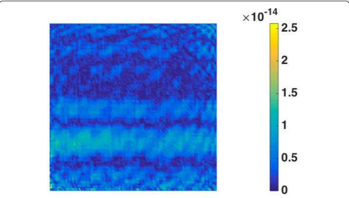
function with small amplitude compared tok. Figure4shows the spatial variation ofε (computed asksep−k). Note thatεcan be reduced by increasing the number of terms
nkinksep. The problem, although, is inverse to the standard homogenization problem: the exact solution here is smooth and the high frequency terms are the errors introduced by the separation. The fact of replacingkbyksepproduces the same error as the opposite. Thus,
ksepis seen as ade-regularizationofk, where the high-frequency terms are truncated. This is the same effect produced in the homogenization, and therefore the error introduced by the homogenization is of the same type of the error produced in using a separated approximation of the material property. Thus, if oscillation terms are included (either by perturbations ofkors) an extra term appears:
esepH =u−usepH ≤ u−uH +uH−usepH ≤CHα+Osc,
being Osc ∝ k−ksepin the case in whichkis replaced byksep. The truncation error,
eM, introduced by PGD is a function decreasing with the number of termsM, so its norm is bounded by eM ≤ CF˜ (M). Note that, as mentioned above, for error affecting the
source termsthe standard estimates for oscillation terms provide a similar expression for Osc [9].
The final error of the PGD solution, therefore can be stated as
u−usepH,M≤CHα+CF˜ (M)+Osc. (6)
This bound expression shows that if Osc dominates over the truncation error, the error of the PGD solution cannot be reduced. On the other hand, if an estimation for Osc and foresepH at enrichment stepiare available, (6) can be used as stopping criteria of the enrichment process.
Problem statement and PGD solution for separated space dimensions
In order to study the propagation of the errors within the PGD scheme a boundary value problem governed by a Poisson equation is considered. Its solutionu, taking values in, satisfies,
−∇ ·(k∇u)=s in (7a)
(k∇u)·n=gN onN (7b)
u=uD onD (7c)
where the source terms, the prescribed values on the Dirichlet boundaryuD, the prescribed flux on the Neumann valuegN and the diffusivitykare the data set. The usual variational form for this problem reads: findu∈V such that
a(u, v)=(v), for all v∈V0, (8)
whereV := {u ∈ H1() :u = uDinD}and its corresponding test functions space is
V0:= {u∈H1() :u=0 onD}. The bilinear and linear formsa(·,·) and(·) are given by
a(u, v) :=
∇u·(k∇v)d and (v) :=
sv d+
N
gNv ds. (9)
Space-separated PGD algorithm
The space-separated PGD algorithm for problem (8) is based on a separated solution
usep(x, y) with the form
u≈usep(x, y)= nu
m=1
Fxm(x)Fym(y).
As usual,usepis inserted in the weak form (8). In this case, the diffusivity functionk(x, y) is also replaced by its separable approximationksep, see Eq. (4), and therefore the operator
a(·,·) is somehow redefined. The problem then reads: findusepsuch that
asep(usep, v)=(v), for all v,
where
asep(u, v) :=
∇u·(k
sep∇v)d.
Using the separability ofusep,ksepand definingv = vxvy(as explained next),asep(·,·) is written (and solved) in terms of one dimensional integrals as,
asep(u, v) := nu m nk l x∇
Fxm·
Gxl∇vx
dx
y∇
Fym·
Gyl∇vy
dy
Note that ifkis not separable, this last step can not be done and the two integrals stay nested.
The definition of(·) remains unchanged.
Assuming that the initialnuterms ofusepare known (that is all functionsFxmandFym, form =1. . .nu are known), each new mode,FxFy, added tousepis obtained by solving the following problem:
asepFxFy, v
=(v)− nu
m=1
asep
FxmFym, v
. (10)
To simplify notation, the dependence of each functionF∗mis kept implicit in the subindex, for exampleFxistands forFxi(x).
The PGD solution is constructed one term at a time using the incremental procedure suggested in (10). The addition of a new term involves solving problem (10) with all the previously computed modes in their right hand side. Note that this problem is non linear because of the multiplication of the unknown functions Fx andFy. This non linearity is usually handled by an alternate-directions algorithm consisting in first solving forFx, assumingFyis known, and then solving forFy, assumingFxis known. These two (linear) subproblems are iterated until convergence.
The test functionsvbelong toV0and they are written asv = δFxFy+FxδFy. When solving the first subproblem,Fyis assumed to be fix and thereforeδFyvanishes. The test functionv, then, simplifies tov=δFxFy. The first subproblem is stated as,
asepFxFy,δFxFy
=(δFxFy)− nu
m=1
asep
FxmFym,δFxFy
. (11)
The second problem is completely symmetric, inverting the dimensionsxandy. Separation of the input data
Several procedures can be applied to obtain separable approximations of known functions. The proper orthogonal decomposition (POD) and the singular value decomposition (SVD) are the most common techniques when the separation is done in two dimensions. Many techniques have been proposed to extend SVD to higher number of dimensions. These techniques are usually calledhigher-order, as they were originally proposed to decompose higher-order tensors. An overview can be found, for example, at [12]. Some examples are thehigher-order SVD(HOSVD) [13], the CANDECOMP/PARAFAC (CP) [14,15] and the Tucker decomposition [16].
When the number of separated dimensions is two, the POD and the SVD are equivalent and they provide a optimal decomposition in the sense that they provide the minimum number of required to obtain an given accuracy. Unfortunately, forn>2 this property is lost and usually there is no guarantee of the optimality of the separated tensor.
Recently in [17] a method based on PGD was proposed to perform efficiently separation of functions. This approach has the advantages of being equivalent to SVD when the separation is done in two-dimensions and it is trivial to extend it to higher dimensions. This technique produced decompositions having lower rank than HOSVD for all tested cases and it does not require to specify the order of the separated function before starting the process (as CP does).
finite element (FE) mesh, that is,fis determined by a set of nodal valuesfifori=1,. . ., nt. In this case the dimensions in which the function will be separated are the cartesian axis
xandy. The form of the approximation is,
f(x, y)≈ q
m=1
αmFm(x)Gm(y),
where the set of functionFm(x) andGm(y) are to be determined. A scalarαmholding the amplitude of each term is added in order to normalizeFmandGm. These functions are also supported in a FE mesh with the corresponding dimensionality; in this example both are 1D meshes.
LetM∈Rm×nbe a matrix with rankrand coefficientsf(xi, yi), wherexiandyiare the nodal locations. The SVD provides a factorisationMin the form
M=U·S·VT (12)
where the columns ofU∈Rm×mare called the left-singular-vectors and denoted here as
Ui. The columns ofV∈Rn×nare called the right-singular-vectors and denotedVj. The matrixS∈ Rm×nis rectangular and diagonal and holds the singular values ofMsorted from larger (S11) to smaller. MatricesUandVare both unitary, in the sense that their transpose its equal to their right inverse.
The factorisation provided be SVD allows to construct a separated representation of the matrixMas,
M=
r
i=1
Sii·Ui·VTi . (13)
In practice, the rank of the separated tensor is kept as low as possible as the computational effort is usually proportional to the number of terms in it. Therefore, it is usual to truncate the sum and discard all terms with amplitud smaller than a given threshold. That is, the terms corresponding to the largest eigenvalues are kept and terms with smaller eigenvalues are discarded.
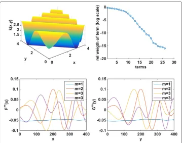
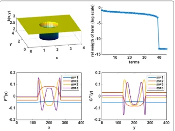
As an example the functionk(x, y)=sin12(x+y)2+2 introduced in (3) is separated using SVD to obtainksep(x, y) as defined in (4). This function is chosen because it does not admits an exact separated representation (Fig.5). Figure5shows the functionk(x, y) (top right), the amplitude of the initial terms in the separated version ofk, that is, the diagonal coefficients of the matrixS(top left), and the functionsFm andGm for the four initial terms ofksep(x, y). Note that with the initial 25 terms the functionk is approximated to machine precision. The meshes corresponding toFandG, both have 402 nodes. Influence of the sampling points
Fig. 5 Separation of the diffusivity function using SVD.Top left panelshows the analytic diffusivity functionk. Top right panelshow the relative weight of the initial 30 terms of the separated functions; the relative weight is computed as the sum of the amplitude of all previous terms, divided by largest amplitude.Lower panels show the functionsFandGcorresponding to the initial four terms
Results
The behaviour of the PGD scheme with respect to errors in the input data is studied next via a series of numerical experiments. The problem (7) is solved using PGD as described above in a square domain with size [0,4]×[0,4]. It is closed with Dirichlet boundary conditions on the top and bottom sides with values one and zero respectively and homogeneous Neumann in the lateral sides. The separated diffusivity function (4) is used. The mesh is structured and regular and has 100 elements in each dimension.
The relative errors shown in convergence curves are computed as theH1norm of the relative difference between the PGD solution and a reference Finite Element solution computed over the same mesh. Note that the FE solution is computed using the exact analytic expression for the diffusivityk.
Input data sampling
The diffusivity function (3) is separated using the SVD approach described in Sect. “Sep-aration of the input data”. To do that, the spatial grid to sample the functionk(x, y) needs to be selected. The first choice taken here is to evaluatekin the same mesh that will be later used in the discretization ofu. In this case, it is a regular grid with 101×101 nodes. This is an overkill mesh to represent the functionk (see first panel of Fig.5). Theksep
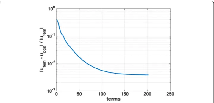
Whenksep is introduced into the weak form and the problem is solved via PGD, the solution obtained is rather inaccurate having relative errors of order 10−2(Fig.6). This poor behaviour comes from the fact that the diffusivity function was sampled at the nodes but it is required by PGD (and by FE) at the integration points. The values ofksepused in the integrals are interpolated spatially and therefore an “H-like” error is introduced. This error is not related with the truncation on the number of terms used inksep, but is only dependent on the grid chosen to samplek.
In the example above, despite the nodal values ofksephave errors that could be negligible, the interpolated values at the mid points of the elements have relative error of order 10−2, coinciding with the maximum accuracy that PGD could provide.
To overcome this limit the grid used to sampleksepis modified so that the grid nodes coincide with the integration points that will be used later by the integrals of PGD. Figure7 shows an example of such a mesh for a quadrature of 4 points per element in each direction
xandy. Same as in the previous grid, the nodal values ofksephave errors comparable of machine tolerance but, in this case, the spatial interpolation is completely avoided. When this newksepis used, the limit imposed by the interpolation disappears and PGD recovers it normal convergence.
Accuracy ofksep
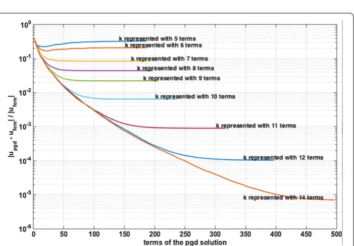
A second set of tests is done to evaluate the relation between the accuracy of PGD and the truncation error ofksep. To do that, the problem is solved several times using different truncated versions ofksepfornk =5,6,7,. . .,11,12,14. Note that allnkare smaller than 26 (26 terms were required to get machine tolerance at the nodes) and therefore we do not expect the errors to vanish at the nodes. The grid forksepis taken coinciding with the integration points. Figure8shows the different convergence curves of the error on the PGD solution as a function of the number of terms. Recall that the errors are computed against the FE solution having the exactkfunction. All curves present a final flattening and a convergence to an error that is imposed by truncation error ofksep. In other words, at some point, the error Osc (that does not depends on the number of terms) dominates
Fig. 7 Grid for the discretization ofksepcoinciding with the location of the integration points.Leftmesh for usepingray linesand location of integration points.Rightmesh forusepinthick gray linesand mesh forksepin thin red lines
Fig. 8 Evolution of the error of the PGD solution with the number of terms. Errors are relative and computed against a FE solution. Eachcurvecorresponds with a PGD solution including a different accuracy ofksep
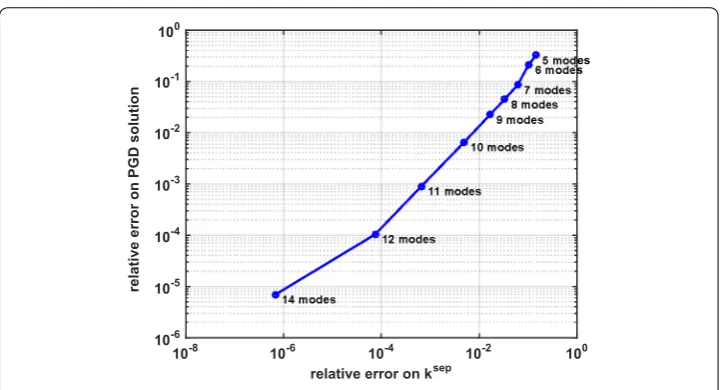
in (6) and therefore the PGD error cannot decrease. The better the description ofksep (that is, the largernk and the smaller the Osc term), the smaller the final error achieved by PGD. For this example and when Osc dominates, the relation between the PGD error andkseptruncation error is linear with slope close to one (as shown in Fig.9).
relative error on ksep
10-8 10-6 10-4 10-2 100
relative error on PGD solution
10-6 10-5 10-4 10-3 10-2 10-1 100
5 modes 6 modes
7 modes 8 modes 9 modes
10 modes
11 modes
12 modes
14 modes
Fig. 9 Dependence of the final PGD error as a function of the errors introduced byksepin the range where the separation error is dominant a linear dependence (having slope equal to one) is obtained
k2(x, y)=
⎧ ⎨ ⎩
2 if (x−2)2+(y−2)2<1
3 otherwise . (14)
The separated version ofk2, shown in Fig.10requires more terms than the smoothkto reach nodal machine precision. The results are consistent with the previous and the final convergence of the PGD solution is controlled by the accuracy ofk2sep. Figure11shows convergence curves fork2sephaving 10, 20, 30, 35 and 40 terms.
Conclusions
The stability of PGD with respect to errors in the input data was studied by means of numerical experiments. These errors are in practice present due to the need of approx-imate input data by truncated separable expressions. Moreover, separation requires dis-cretization introducing into the input data a “spatial” h-like error.
Results show that PGD is stable (it does not amplify errors). In the tested case of a boundary value problem governed by the Poisson equation, the errors introduced on the diffusivity function are linear with the final error that PGD commits. The grid in which the separated data is represented is crucial to the accuracy of PGD; to minimize interpolation error, the mesh for the input data should coincide with the integration points used for the solution ofu.
The relation between the errors in the input data and the final error of PGD can be used to decide the accuracy required in the input data to get a certain accuracy on the PGD solution. In the example presented in this work, as the relation between these errors is linear, it is straightforward to determine, given the desired accuracy in the final solution, which is the accuracy required at the nodal values in the input data.
Fig. 10 Separation of the discontinuous diffusivity function using SVD.Top left panelshows the analytic diffusivity functionk2.Top right panelshow the relative weight of the initial 45 terms of the separated function; the relative weight is computed as the sum of the amplitude of all previous terms, divided by largest amplitude.Lower panelsshow the functionsFandGcorresponding to the initial four terms
Fig. 11 Dependence of the final PGD error as a function of the errors introduced by the discontinuous diffusivity functionk2sep
Authors’ contributions
All authors discussed the content of the article based on their previous experiences using PGD. SD and PD prepare and run the numerical examples based on the Poisson problem. EC and DG prepare and run the numerical examples based on the XXX problem. All authors read and approved the final manuscript.
Author details
1Laboratori de Calcul Numeric (LaCaN), E.T.S. de Ingenieros de Caminos, Canales y Puertos, Universitat Politecnica de Catalunya, Jordi Girona 1, 08034 Barcelona, Spain,2Aragon Institute of Engineering Research, Universidad de Zaragoza, María de Luna, s.n., 50018 Zaragoza, Spain.
Acknowledgements
This work has been partially supported by the Spanish Ministry of Science and Competitiveness, through Grant Number CICYT- DPI2014-51844-C2-2-R and DPI2014-51844-C2-1-R and by the Generalitat de Catalunya, Grant Number 2014-SGR-1471.
Competing interests
The authors declare that they have no competing interests.
Received: 11 May 2015 Accepted 5 November 2015
References
1. Ammar A, Mokdad B, Chinesta F, Keunings R. A new family of solvers for some classes of multidimensional par-tial differenpar-tial equations encountered in kinetic theory modelling of complex fluids. J Non Newton Fluid Mech. 2006;139:153–76.
2. Ammar A, Mokdad B, Chinesta F, Keunings R. A new family of solvers for some classes of multidimensional partial differential equations encountered in kinetic theory modeling of complex fluids. Part II: transient simulation using space-time separated representations. J Non Newton Fluid Mech. 2007;144:98–121.
3. Ammar A, Huerta A, Chinesta F, Cueto E. Parametric solutions involving geometry: a step towards efficient shape optimization. Comput Methods Appl Mech Eng. 2014;268:178–93.
4. Zlotnik S, Díez P, Modesto D, Huerta A. Proper generalized decomposition of a geometrically parametrized heat problem with geophysical applications. Int J Numer Meth Eng. 2015;103(10):737–58. doi:10.1002/nme.4909. 5. González D, Cueto E, Chinesta F. Real-time direct integration of reduced solid dynamics equations. Int J Numer Meth
Eng. 2014;99(9):633–53.
6. Ammar A, Chinesta F, Díez P, Huerta A. An error estimator for separated representations of highly multidimensional models. Comput Methods Appl Mech Eng. 2010;199:1872–80.
7. Bouclier R, Louf F, Chamoin L. Real-time validation of mechanical models coupling PGD and constitutive relation error. Comput Mech. 2013;52(4):861–83.
8. Nadal E, Leygue A, Chinesta F, Beringhier M, Ródenas JJ, Fuenmayor FJ. A separated representation of an error indicator for the mesh refinement process under the proper generalized decomposition framework. Comput Mech. 2015;55(2):251–66.
9. Morin P, Nochetto RH, Siebert KG. Data oscillation and convergence of adaptive FEM. SIAM J Numer Anal. 2000;38(2):466–88.
10. Abdulle A. On a priori error analysis of fully discrete heterogeneous multiscale FEM. Multiscale Modeling and Simula-tion. SIAM Interdiscip J. 2005;4(2):447–59.
11. Ming P, Zhang P. Analysis of the heterogeneous multiscale method for elliptic homogenization problems. J Am Math Soc. 2005;18(1):121–56.
12. Kolda TG, Bader BW. Tensor decompositions and applications. SIAM Rev. 2009;51(3):455–500.
13. De Lathauwer L, De Moor B, Vandewalle J. A multilinear singular value decomposition. SIAM J Matrix Anal Appl. 2000;21(4):1253–78.
14. Carroll JD, Chang J-J. Analysis of individual differences in multidimensional scaling via an n-way generalization of “Eckart-Young” decomposition. Psychometrika. 1970;35(3):283–319.
15. Harshman RA. Foundations of the PARAFAC procedure: models and conditions for an “explanatory” multimodal factor analysis. UCLA Work Pap phon. 1970;16:1–84.
16. Tucker LR. Some mathematical notes on three-mode factor analysis. Psychometrika. 1966;31:279–311.
17. Modesto D, Zlotnik S, Huerta A. Proper generalized decomposition for parameterized helmholtz problems in hetero-geneous and unbounded domains: application to harbor agitation. Comput Methods Appl Mech Eng. 2015. doi:10.