R E S E A R C H
Open Access
Efficient influence spread estimation for
influence maximization under the linear
threshold model
Zaixin Lu
*, Lidan Fan, Weili Wu, Bhavani Thuraisingham and Kai Yang
*Correspondence: [email protected]
Department of Computer Science, University of Texas at Dallas, 800 W. Campbell Road, Richardson, TX 75080, USA
Abstract
Background: This paper investigates the influence maximization (IM) problem in social networks under the linear threshold (LT) model. Kempe et al. (ACM SIGKDD Conference on Knowledge Discovery and Data Mining, pp. 137–146, 2003) showed that the standard greedy algorithm, which selects the node with the maximum marginal gain repeatedly, brings ae−e1-factor approximation solution to this problem. However, Chen et al. (International Conference on Data Mining, pp. 88–97, 2010) proved that the problem of computing the expected influence spread (EIS) of a node is #P-hard. Therefore, to compute the marginal gain exactly is computational intractable. Methods: We step-up on investigating efficient algorithm to compute EIS. We show that the EIS of a node can be computed by finding cycles through it, and we further develop an exact algorithm to compute EIS within a small number of hops and an approximation algorithm to estimate EIS without the hop constraint. Based on the proposed EIS algorithms, we finally develop an efficient greedy based algorithm for IM. Results: We compare our algorithm with some well-known IM algorithms on four real-world social networks. The experimental results show that our algorithm is more accurate than others in finding the most influential nodes, and it is also better than or competitive with them in terms of running time.
Conclusions: IM is a big topic in social network analysis. In this paper, we investigate efficient influence spread estimation for IM under the LT model. We develop two influence spread estimation algorithms and a new greedy based algorithm for IM under the LT model. The performance of the proposed algorithms are analyzed theoretically and evaluated through simulations.
Keywords: Social network analysis; Expected influence spread estimation; Influence maximization; Linear threshold model
Background
Social network is a multidisciplinary research area for both academia and industry, including social network modeling, social network analysis, and data mining. An inter-esting problem in social network analysis is influence maximization (IM), which can be applied in marketing to deploy business strategies. Typically, IM is the problem that given a graphGas a social network, an influence spread model and an integerkselect the top
knodes as seeds to maximize the expected influence spread (EIS) throughG. One corre-sponding issue in marketing is product promotion. In order to advertise a new product efficiently within a limited budget, a company may choose a few people as seeds who will be given free samples. It is likely that those people will recommend others, such as their friends, relatives or co-workers, to try this product. Eventually, a great number of people may adopt the product due to such ‘word-of-mouth’ effect [1-6]. Intuitively, the initial seed selection is a key factor that will impact on the success of the product promo-tion. Therefore, it is important to design applicative influence spread model and efficient search algorithm to find the most influential people in social networks.
IM was first investigated as an combinatorial optimization problem by Kempe et al. in [5]. They considered two influence spread models, namely, Independent Cascade (IC; [2,3]) and Linear Threshold (LT; [7,8]), and proved a series of theoretical results. After that, the two models have been extensively studied (please see, e.g., [9-15] for recent works). In this paper, we focus upon the LT model. LetSbe a set of initially active nodes; the influence, under the LT model, propagates in a threshold manner. That is, a nodevis activated if and only if the sum of influence it receives from its active neighbors exceeds a thresholdλ(v)chosen uniformly at random.
As we understand, a crucial part of IM is how to compute the EIS given a node, since only we know the EIS of each node, and then we could find a seed set to maximize the combinatorial EIS. The exact EIS computation was left as an open problem in [5] and has attracted a great deal of attentions in recent years (see, e.g., [9-11,13,15,16]). In [11], Chen et al. proved that computing the exact EIS under the LT model is #P-hard. Therefore, a polynomial time exact solution does not exist unlessP =NP. But based on the observa-tions in [11,15], the influence diminishes rapidly during the diffusion in many real-world social networks under the LT model. In other words, the influence spread of a seed is lim-ited within a small number of hops. It has been shown that the influence spread under the LT model can be computed by searching simple paths starting from the seeds [11,15]. Therefore, we can define a hop constraintTsuch that given a seedv, we only take paths withinThops to estimate the EIS ofv. The main contributions of this paper are as follows:
1. We develop an exact algorithm for computing the EIS within four hops. Instead of finding simple paths, we compute the EIS of a node by finding cycles through it. In this study, a cycle of lengthlis defined as a path visiting a node twice and visiting otherl−2nodes exactly once. The detailed algorithm is given in the ‘Methods’ section.
2. For the case thatT >4, we develop an approximation algorithm to estimate EIS based on random walk. The experimental results in the ‘Results and discussion’ section show that more precise and quick results can be obtained by using a combination of our exact and approximation algorithms rather than using methods based on simple path.
The update algorithms are represented in the ‘Influence maximization’ section. It is able to say that the two lists contain all the information for doing the seed
selection, and they can be easily and quickly updated by our update algorithms.
4. We compare our algorithm with some well-known IM algorithms on four real-world social networks. The experimental results show that our algorithm is more accurate than others in finding the most influential nodes, and it is also better than or competitive with them in terms of running time.
The rest of this paper is organized as follows: The ‘Related work’ section intro-duces the related works. ‘Problem description’ section gives the problem descrip-tions of both EISE and IM. ‘Methods’ and ‘Influence maximization’ secdescrip-tions study the two problems, respectively. In detail, ‘A deterministic algorithm’ section effi-ciently solves the EISE assuming that the influence spread is negligible after four hops. ‘A randomized algorithm’ section presents an approximation algorithm for general EISE. The ‘Influence maximization’ section presents a fast method to solve IM by using the algorithms proposed in the ‘Methods’ section. Finally, ‘Results and discussion’ section gives the simulation results, and the ‘Conclusion’ section concludes this paper.
Related work
In the literature, the IM problem has been extensively studied under the IC and LT mod-els. Kempe et al. in [5] first showed that it is NP-hard to determine the optimum for IM under the two models, and by showing that the EIS function is monotone and submod-ular, they proved that the standard greedy algorithm brings a e−e1-factor approximation solution. In mathematics, a set functionf : 2 = R+is monotone and submodular if ∀S2⊆ S1, we havef(S1)≥f(S2)andf(S1∪ {u})−f(S1)≥f(S2∪ {u})−f(S2), whereu is an arbitrary item. In such cases, a e−e1-factor approximation solution can be obtained by picking the item with the maximum marginal gain repeatedly [17]. In [5], how to com-pute the exact marginal gain (i.e., comcom-pute the EIS increment when adding a node) under the two models was left as an open problem, and they estimated it by running the Monte Carlo (MC) simulation, which is not computational efficient (e.g., it takes days to select 50 seeds in a moderate size graph of 30K nodes [11]). Motivated by improving the run-ning time performance, many algorithms have been proposed. Leskovec et al. developed a Cost-Effective Lazy Forward (CELF) algorithm, which is up to 700 times faster than the greedy algorithm with Monte Carlo simulation [16]. But as the results shown in [9], CELF still cannot be applied to find seeds in large social networks, and it takes several hours to select 50 seeds in a graph with tens of thousands of nodes. To further reduce the running time, Goyal et al. [13] developed an extension of CELF, called CELF++, which was showed 0.35 to 0.55 faster than CELF. In [9], Chen et al. proposed two new greedy algorithms, namely NewGreedy and MixedGreedy. NewGreedy reduces the running time by deleting edges having no contribution to influence spread (similar idea was also proposed in [18]), and MixedGreedy which is a combination of NewGreedy and CELF (it uses NewGreedy as the first step and applies CELF for the remaining rounds). Based on the experiments, they showed that MixedGreedy is much faster than both NewGreedy and CELF.
The efficiency of MIA was demonstrated in [10]. Besides selecting nodes greedily, Wang et al. [19] proposed a community-based algorithm for mining the topkinfluential nodes under the IC model, and Jiang et al. in [14] proposed a heuristic algorithm based on Simulated Annealing.
In terms of LT model, after Kempe et al. proposed the greedy algorithm [5], the most recent works for IM under this model are [10,12,15]. In [10], Chen et al. proved that the EIS under LT model can be computed in linear time in a directed acyclic graph, and they proposed an algorithm called Local Directed Acyclic Graph (LDAG). Given a general graph, it first converts the original graph into small acyclic graphs, and it only consid-ers the EIS of a node within its local graph when computing the marginal gain. In [12], Narayanam and Narahari developed an algorithm for the LT model that selects the nodes based on the Shapley Value. In [15], Goyal et al. proposed an algorithm called SIMPATH, which estimates the EIS by searching for the simple paths starting from seeds. Since it is computationally expensive to find all the simple paths, they adopted a parameterηto prune them. They also applied the vertex cover optimization to cut down the number of iterations. Based on their experimental results, SIMPATH showed its merits from the aspects of running time and seed quality.
Problem description
Many introductions about the LT model and IM problem can be found in detail in papers cited above. Here, for the sake of completeness, we give a brief description for the LT model and formal definitions for IM and EISE.
Definition 1. LetG(V,E)be a directed graph; we define
• Nin(v)(respectivelyNout(v)) to be the set of incoming (respectively outgoing) neighbors ofv(∀v∈V).
• λ(v)to be the threshold ofv, which is a real number in the range of[0, 1]chosen uniformly at random.
• x(v)to be a 0 to 1 variable which indicates whethervis active or not.
According to Definition 1, given a weighted directed graphG(V,E,w), wherew(e) ∈ [0, 1] (∀e∈ E) is a weight function, the sum of influencevreceives can be formulated as
u∈Nin(v)x(u)w(u,v). Without loss of generality, we assume
u∈Nin(v)w(u,v) ≤1 (∀v∈
V). In the LT model, time is discrete. Given a seed setS, at time 0, we have ∀v ∈ S, x(v) = 1, and∀u ∈ (V\S),x(u) = 0. At any particular timet, a nodev ∈ V becomes active ifu∈Nin(v)x(u)w(u,v)≥λ(v). Finally, the influence spread process stops at a time slot when there is no newly activated node.
Definition 2.EISE: Given a weighted directed graphG(V,E,w) and a setS ⊆ V of nodes, EISE is the problem of estimating the expected number of active nodes at the end of the influence spread. EISET is the problem that given an integerT, estimates the
expected number of nodes that are active at timeT.
For the rest of this paper, given a seed setS, we denote byσ(S)the expected number of nodes that are eventually active and denote byσT(S)the expected number of nodes
the probability distributions of active nodes givenSandσT(S)is a time limited version
ofσ(S).
Definition 3.IM:Given a weighted directed graphG(V,E,w)and a parameterk, the IM problem is to find a seed setSof cardinalitykto maximizeσ(S).
As the experimental results shown in [15], under the LT model, the EIS is negligible after a small number of hops (usually three or four hops) in many real-world social networks. Therefore, to solve the IM problem, it is sufficient to computeσT(S)instead ofσ(S)for
some small value ofT.
Methods
We first present a deterministic algorithm for computing the exact value ofσT(v)for the
case thatT ≤4 in the ‘A deterministic algorithm’ section and then present a randomized algorithm for estimatingσT(v)forT≥5 in the ‘A randomized algorithm’ section.
Definition 4.In this study, we define
• a path is a sequence of nodes, each of which is connected to the next one in the sequence; and a path with no repeated nodes is called a simple path.
• a cycle is a path such that the first node appears twice and the other nodes appear exactly once; and a simple cycle is a cycle such that the first and last nodes are the same.
A deterministic algorithm
According to the observation in [15], the EIS of a nodevafter three or four hops is neg-ligible in most cases. Therefore, we are interested in how to computeσT(v)forT ≤4. In
[11], it has been shown that the EIS of a seed setSunder the LT model can be formulated as
σ(S)=
π∈P(S)
e∈π
w(e)+ |S| [ 15] ,
whereP(S)denotes the set of simple paths starting from nodes inS,πdenotes an element inP(S), andedenotes an edge inπ. Thus,∀v∈V, we have
σ(v)=
π∈P(v)
e∈π
w(e)+1,
whereP(v)denotes the set of simple paths starting from nodev.
As an example shown in Figure 1, consideringv0is an active node, then the probability thatv4can be activated byv0isw(0, 1)w(1, 4)+w(0, 2)w(2, 4)+w(0, 3)w(3, 4), which is
v
1v
4v
2v
0v
3the sum of weight products of all the simple paths fromv0tov4. Although the example is easy to understand, in a general graphG, it requires exponential time to enumerate all the simple paths. Thus, to compute the exact value ofσ(v)is computational intractable, and a hop constraintTis used in this paper to balance the accuracy of EISE and the program efficiency in terms of running time.
In order to find a nodevwith the maximumσT(v), we have to computeσT(v)for all
the nodesv∈ V. Letσ0(v) = 1 (∀v∈ V); we first consider the simple case thatT = 1. In such cases, we haveσ1(v) = σ0(v)+u∈Nout(v)w(v,u), because there is only direct
influence spread without propagation. WhenT>1, we can computeσT(v)by recursively
finding all the simple paths of length no more thanT, starting fromv, which requires O(T) time by using the depth-first search (DFS) algorithm, anddenotes the node maximum degree. Thus, letGbe a weighted directed graph; computingσT(v)for all the
nodes inGrequiresO(nT)time if we use the above simple path method [15], wheren
denotes the number of nodes inG. To further improve the running time performance, we develop a dynamic programming (DP) approach to computeσT(v)forT ≤4. It is based
on searching cycles instead of simple paths.
As an example shown in Figure 2, there are three types of cycles of length 4, and only the third one is a simple cycle. LetCl(v)denote the set of cycles of lengthl, starting from
v, and let
T(v)=
l=2···T
π∈Cl(v)
e∈π
w(e),
we have
σT(v) = σ0(v)+
u∈Nout(v)
w(v,u)·(σV\v T−1(u))
= σ0(v)+
u∈Nout(v)
w(v,u)·(σT−1(u))
−T(v),
whereσTV−\v1(u)denotes the EIS of nodeuin the induced graph ofV\vwithinT−1 hops, andT(v)denotes the invalid influence spread involving cycles.
v
1v
2v
0(III)
v
3v
1v
2v
0(II)
v
3v
1v
2v
0(I)
v
3v
1v
3v
2v
0v
4Figure 3 An illustration of computing3(v0).
Figure 3 shows an example, in whichv3andv4arev0’s outgoing neighbors. It is easy to seeσ2(v3)=1+w(3, 0)+w(3, 1)+w(3, 0)w(0, 4)andσ2(v4)=1. Thus,
σ0(v0)+
u∈Nout(v0)
w(v0,u)·(σ2(u))
= w(0, 3)+w(0, 4)+w(0, 3)w(3, 0)+w(0, 3)w(3, 1) +w(0, 3)w(3, 0)w(0, 4)+1,
in which the termsw(0, 3)w(3, 0)andw(0, 3)w(3, 0)w(0, 4)have to be removed since they involve cycles. The rest of this section is devoted to investigating how to computeT(v)
forT ≤4.
Lemma 1.Given a weighted directed graph G(V,E,w)and an arbitrary node v ∈ V , T(v)can be computed in O
2time when T≤4.
A brief description for the idea of our method is presented before the formal algo-rithm and its proof. Firstly, T(v) involves all the cycles of length no more than T,
starting fromv. In order to compute 4(v) efficiently, we divide4(v)into three parts:
π∈Cl(v)
e∈πw(e) (l = 2, 3, 4) to carry on the analysis. If each part can be
com-puted in O(2) time, 4(v), which is the sum of them, can be obtained in O(2) time. Secondly, considering Cl(v) (2 ≤ l ≤ 4), we can further classify the cycles in Cl(v) into l − 1 types. Note that a cycle of length l, starting from v, consists of a
sequence ofl+1 nodes, two of which arevand others are distinct. Therefore, we can label a cycle according to the position in the sequence where the second v appears. ∀v ∈ V, let CTl(v) denote the set of cycles of length T, whose lth node is v, we have
T(v) =
l=2,···,T
π∈Cl(v)
e∈π
w(e)
=
l=2,···,T
l=3,···,l+1
π∈Cl l(v)
e∈π
w(e).
In order to compute T(v), our method will compute each π∈Cl l(v)
e∈πw(e)
separately.
Proof.We will prove Lemma 1 by showing thatπ∈C
l(v)
e∈πw(e)can be computed in
O(2)time whenl=4, and for the case thatl<4,
π∈Cl(v)
e∈πw(e)can be computed
Consider case (I). Such a cycle consists of a simple cycle of length 2 and a simple path of length 2. LetP2(v)denote the set of simple paths of length 2, starting fromv, andC23(v) denote the set of simple cycles of length 2 throughv.P2(v)can be obtained inO(2)time by DFS, andC23(v)can be obtained by finding the set of nodes that are both incoming and outgoing neighbors ofv, i.e.,
C3 2(v)=
(v,u,v):u∈Nout(v)∩Nin(v) .
The intersection of two lists can be obtained in linear time if the two lists are sorted. LetI(v)=Nout(v)∩Nin(v)andκ=u∈I(v)w(v,u)w(u,v); we have
π∈C3 4(v)
e∈π
w(e)
=
π∈P2(v)
u∈I(v)\π
w(v,u)w(u,v)
e∈π
w(e)
=
π∈P2(v) ⎛
⎝κ−
u∈π∩I(v)
w(v,u)w(u,v) ⎞
⎠
e∈π
w(e)
=
π∈P2(v)
⎛
⎝κ−
u∈π\v
w(v,u)w(u,v) ⎞
⎠
e∈π
w(e),
in whichI(v)\π denotes the set of nodes inI(v) but not inπ, e ∈ π denotes an edge in π, andu ∈ π denotes a node inπ. Note that ifu ∈ I(v), we have (v,u) ∈ E or (u,v) ∈ E. In such cases, w(v,u)w(u,v) = 0. Therefore, u∈π∩I(v)w(v,u)w(u,v) =
u∈π\vw(v,u)w(u,v). Since P2(v) consists of at most 2 elements, each of which includes only two edges,π∈P2(v)(κ −u∈π\vw(v,u)w(u,v))e∈πw(e)can be com-puted inO(2)time.
Consider case (II).π∈C4 4(v)
e∈πw(e)can be computed by a similar method. A cycle in
C4
4(v)consists of a simple cycle of length 3, in which the first and last nodes arev. There-fore, instead of directly constructing a set of simple cycles of length 3, we can construct a setP2(v)of simple paths of length 2. Letl(π)denote the last node of a pathπ ∈P2(v) and letτ =u∈Nout(v)w(v,u); we have
π∈C4 4(v)
e∈π
w(e)
=
π∈P2(v)
w(l(π),v) ⎛
⎝
u∈Nout(v)\π
w(v,u) ⎞
⎠
e∈π
w(e)
=
π∈P2(v)
w(l(π),v) ⎛
⎝τ −
u∈π\v
w(v,u) ⎞
⎠
e∈π
w(e),
in whichw(l(π),v) = 0 ifl(π) ∈ Nin(v). Therefore,π∈C4 4(v)
e∈πw(e) can also be
computed inO(2)time.
Consider case (III). The analysis is somewhat more complicated. Instead of comput-ing π∈C5
4(v)
e∈πw(e) directly, we first show that
π∈(C5 4(v)∪C(v))
e∈πw(e) can be
v0
v1
v2
Figure 4 An invalid case.
ρ2(v,v)=u∈Nout(v)∩Nin(v)w(v,u)w(u,v
). LetN2
out(v)be the set of nodes that are reach-able fromvwith exact two hops. To computeρ2(v,v)for all the nodesv ∈ Nout2 (v), we can build up an outgoing tree rooted atv, in which the nodes are repeatable among dif-ferent paths. This can be done inO(2)time by DFS. In addition, letNin2(v)be the set of nodes that can reachvwith exact two hops, we can build up an incoming tree rooted atv to computeρ2(v,v)for all the nodesv∈Nin2(v)in the same way. Then, we have
π∈C5 4(v)∪C(v)
e∈π
w(e)
=
v∈N2
out(v)∩Nin2(v)
ρ2(v,v)ρ2(v,v),
which can be computed inO(2)time. It is easy to see
π∈C5 4(v)
e∈π
w(e)
=
π∈C5 4(v)∪C(v)
e∈π
w(e)−
π∈C(v)
e∈π
w(e).
Therefore, to showπ∈C5 4(v)
e∈πw(e)can be computed inO(2)time, it is sufficient
to show thatπ∈C(v)e∈πw(e)can be computed inO(2)time. We have
π∈C(v)
e∈π
w(e)
=
v∈I(v)
u∈I(v)
w(v,v)w(v,u)w(u,v)w(v,v),
where I(v) = Nout(v) ∩ Nin(v) and I(v) = Nout(v) ∩ Nin(v). Therefore,
π∈C(v)e∈πw(e)can be computed inO(2)time.
In sum, we proveπ∈C4(v)e∈πw(e)(∀v∈V) can be computed inO(2)time. It can be shown thatπ∈Cl(v)e∈πw(e)(l < 4) can be computed inO(2)time or less by a similar method. Therefore, it requires onlyO(2)time to compute4(v)(∀v∈V).
Algorithm 1EISE4
0: input: a weighted directed graphG=(V,E,w).
1: letσ1(v)=
u∈Nout(v)wv,u(∀v∈V); 2: forl=2· · ·4do
3: σl(v)=σ1(v)−l(v)+u∈Nout(v)wv,u·σl−1(u); 4: end for
5: output: a list ofσ4(v)for all the nodesv∈V.
Proof. Without considering the possible numerical computation error, the solution of Algorithm 1 is exact, and the time complexity analysis easily follows the algorithm. The computation ofσl(v)only depends onσl−1(u)(u ∈ Nout(v)) andl(v). Therefore,σ4(v) for all the nodesv∈Vcan be computed by a DP approach. The number of subproblems is O(n)and each subproblem can be solved inO(2)time. Therefore, Algorithm 1 requires O(n2)time.
Compared with the method based on a simple path, which requiresO(4)time to com-puteσ4(v)for a nodev, the core advantage of Algorithm 1 is its running time performance. Based on our experiments in the ‘Results and discussion’ section, whenT≤4, Algorithm 1 can compute theσT(v)for all the nodes in a moderate size graph in about 1 s.
A randomized algorithm
Theorem 1 shows that Algorithm 1 can efficiently computeσ(v), if the EIS from nodev is negligible after four hops. For the case that the EIS within a large numberT hops is not negligible, it has been shown that computingσT(v)is #P-hard [11]. To estimateσT(v)
approximately, we can use MC simulation, i.e., simulate the influence spread process a sufficient number of times, re-choosing the thresholds uniformly at random, and use the arithmetic mean of the results instead of the EIS. LetX1,X2,· · ·,Xr be the numbers of
active nodes at timeT forrruns, and letE[X] be the EIS within timeT. By Hoeffding’s inequality [20], we have
Pr|X−E[X]| ≥≤exp
−r 22r2 i=1(bi−ai)2
,
whereaiandbiare the lower and upper bounds forXi, respectively. Apparently,ai ≥ 0
andbi ≤ n, wheren is the number of nodes in the graph. Thus,∀0 < δ < 1, when
r≥ n2ln21δ, the probability that|X−E[X]| ≥is at mostδ. Therefore, the EIS estimated
by using MC simulation with a sufficient number of runs is nearly exact. However, as the experiments shown in [5,11,15], applying the MC simulation to estimate the EIS is computational expensive, and the standard greedy algorithm with MC simulation (run 10,000 times to get the average) requires days to select 50 seeds in some real-world social networks with tens of thousands of nodes.
To improve the computation efficiency, we developed a randomized algorithm, com-puting σT(v) forT ≥ 5. We first give the main idea of our method. Recall that the
EIS of a node v can be computed by searching simple paths starting from v; thus, σT(v) = π∈PT(v)
all the elements π ∈ PT(v), and let | · | be the number of elements in ‘·’; we have
σT(v) = avg(PT(v))|PT(v)|. However, obtaining avg(PT(v))and |PT(v)| requires the
knowledge ofPT(v)and is therefore as difficult as the original problem. We propose an
alternative approach. Instead of computingσT(v)directly, we relaxPT(v)toP´T(v)that
contains all the paths starting fromv, instead of simple paths. Letx(π ∈PT(v))be a 0 to
1 variable denote whetherπis a simple path or not; we have
σT(v)=
π∈ ´PT(v)
xπ∈PT(v) e∈π
w(e).
The next question is how to estimate avg(P´T(v))and| ´PT(v)|to obtainσT(v).
Lemma 2.Given a directed graph G(V,E)and an integer T, there is a polynomial time algorithm to compute| ´PT(v)|for all the nodes v∈V .
Proof.We can compute| ´PT(v)|by iteration or recursion.∀1≤l≤T, we have
| ´Pl(v)| = |Pl(v)| = |Nout(v)|, l=1 | ´Pl(v)| =u∈Nout(v)| ´Pl−1(v)|, otherwise.
| ´P1(v)| equals to the number of outgoing neighbors ofv, and| ´Pl(v)| (l > 1) can be
obtained by a DP approach. Since there areO(nT)subproblems and each subproblem can be solved inO()time,| ´PT(v)|can be obtained inO(nT)time.
Theorem 2. Letandδbe two positive constants in the range of(0, 1). There is a random walk algorithm such that given a weighted directed graph G(V,E,w)and a node v ∈ V , it gives a(1±)-factor approximation solution to avg(P´T(v))in O
1
2ln1δ+nT
time with probability greater than1−δ.
Proof.We can use uniform random sampling, which selects elements with equal prob-ability fromP´T(v). By Lemma 2, we can obtain| ´PT(v)|for all the nodesv∈VinO(nT)
time. Let the probability Pr(yi+1 = u|yi = u) = | ´PT−i(u )|
| ´PT−i+1(u)| and Pr(y1 = v) = 1;
then, a path of lengthT can be generated by takingT successive random steps.∀a path π=(v1,v2,· · ·,vT)inP´T(v), we have
Pr(π) =
i=1,···,T−1
Pr(yi+1=vi+1|yi=vi)
=
i=1,···,T
| ´PT−i(vi+1)| | ´PT−i+1(vi)|
= 1
| ´PT(v)|
.
Therefore, we can generate pathsπ1,π2,· · ·,πr uniformly at random. By Hoeffding’s
inequality, we have
Pr
|
i=1,···,r
e∈πiw(e)r
− avg
´
PT(v) | ≥ ≤exp ⎛ ⎜
⎝− 22r2
r i=1
maxπ∈ ´P
T(v)
e∈πw(e)
where maxπ∈ ´P
T(v)
eπw(e)is the maximum weight product of a path of lengthTstarting
fromv. Sincew(e)≤1 (∀e∈E), we have maxπ∈ ´P
T(v)
eπw(e)≤1. Thus, Theorem 2 is
proved.
Based on Theorem 2, we now describe our randomized algorithm for computingσT(v)
for all the nodesv∈V. It runs inO(nT+nr)time, whereris a constant and does not depend on the input graph.
In Algorithm 2, it first computes| ´PT(v)|(step 1) and then estimatesσT(v)by uniform
random sampling. As far as the running time, the most time-consuming part is steps 2 to 8, in whichris independent of the input graph. It is clear that whenris small, the accuracy of EISE is low, but the estimation time is short, and vice verse. Compared with MC simulation, Algorithm 2 is much faster. In order to estimate the EIS of a node, it only generates a constant number of paths, while if MC simulation is applied instead of Algorithm 2, each time we have to re-choose the thresholds for all the nodes, and the time complexity isO((|V| + |E|)r), when most of the edges are accessed each time. In the experiment, we observed that the error is less than 3% whenT =5, using an appropriate number of samples (r=1, 000).
Algorithm 2EISET
0: input: a weighted directed graphG=(V,E,w)and two integersT andr.
1: construct| ´Pl(v)|(1≤l≤T) for all the nodesv∈V;
2: forv∈Vdo
3: letσT(v)=0;
4: fori=1,· · ·,rdo
5: letπrbe the path of lengthT, generated by the random walk technique;
6: σT =σT+x(πr∈PT(v))e∈πrw(e); 7: end for
8: end for
9: σT(v)=σT(v)| ´Plr(v)|;
10: output: a list ofσT(v)for all the nodesv∈V.
Influence maximization
Considering the computational efficiency, we define a hop constraint for EISE, and we present two algorithms in ‘Methods’ section to computeσT(v)inv’s local area (T hops).
The proposed algorithms are worth applying to solve the IM problem greedily. Given a weighted directed graphG(V,E,w), the standard greedy algorithm will run EISEO(n) times to select a seed, wherendenotes the number of nodes. To further reduce the run-ning time, we construct an influence listIL to store the EIS of nodes in the induced graph ofG\S, whereSis the current seed set. Letv1,v2,· · ·,vnbe the nodes in the input
graph. Given a parameterT, initially we have IL= {l1=σT(v1),· · ·,ln =σT(vn)}, since
S= ∅. After adding a nodeviintoS, all the nodes, whose local area includevi, have to be
Algorithm 3UpdateIL
0: input:G=(V,E,w),v,S, and IL.
1: construct an incoming tree of depth T rooted at vin the induced graph of G\S
(without loss of generality, assume that the simple paths areπ1,π2,· · ·,πm);
2: fori=1· · ·mdo
3: leti0,i1,· · ·,iT be the nodes visited byπi sequentially andli0,li1,· · ·,liT be the
corresponding elements in IL (in whichi0=v);
4: forj=1· · ·Tdo
5: lij =lij− j
l=1w(il,il−1)(1+σ
V\S\{i1,···,ij} T−j (v));
6: end for
7: end for
8: output: IL.
In Algorithm 3, the incoming tree is node repeated, including all the simple path of lengthTending atv.jl=1w(il,il−1)denotes the EIS fromijtoi0via path(ij,ij−1,· · ·,i0),
where i0 = v, and σ
V\S\{i1,···,ij}
T−j (v) denotes the EIS of v in the induce graph of
V\S\{i1,· · ·,ij}. Thus, j
l=1w(il,il−1)(1+σ
V\S\{i1,···,ij}
T−j (v))denotes the entire influence
diffused fromijthrough path(ij,ij−1,· · ·,i1,π), whereπis a path of length no more than T−jstarting fromvand does not contain any node in{i1,i2,· · ·,ij}. It is clear that after
steps 2 to 7,∀u ∈ (V\S), the influence diffused fromuthroughvis removed from the corresponding element in IL. Consider now the running time. Algorithm 3 generates at mostO(j)nodes in depthj(1≤j≤T). For each nodeijin depthj,σTV−\Sj\{i1,···,ij}(v)can
be computed by building an outgoing tree of depthT−jrooted atv, which can be done by DFS inO(T−j)time. Therefore, Algorithm 3 runs inO(T)time, consideringTas a constant. Compared with running EISE for all the nodes, it is much faster whenTand are relatively small.
In addition to IL, we construct another list, namely, probability list PL, to store the nodes’ active probabilities at timeT. WhenS= ∅, obviously PL= {p1=0,· · ·,pn=0}.
Similarly, after adding a nodeviintoS, the active probabilities of nodes invi’s local area
need to be updated. The algorithm of updating PL is given in Algorithm 4.
Algorithm 4UpdatePL
0: input:G=(V,E,w),v,S, and PL.
1: construct an outgoing tree of depth T rooted at v in the induced graph of G\S (without loss of generality, assume the simple paths areπ1,π2,· · ·,πm);
2: fori=1· · ·mdo
3: leti0,i1,· · ·,iT be the nodes visited byπisequentially andpi0,pi1,· · ·,piT be the
corresponding elements in PL; 4: forj=1· · ·Tdo
5: pij =pij+(1−pv) j−1
l=0w(il,il+1); 6: end for
7: end for
Algorithm 4 searches the simple paths of lengthTstarting fromvand updates the active probability of a nodeijaccording to step 5, in whichjl−=10w(il,il+1)is the influence spread fromvtoijthrough path(i0,· · ·,ij), and 1−pvis the increment ofv’ active probability
when it is added intoS. In the outgoing tree, there are O(T)nodes; thus, PL can be updated inO(T)time.
Assume vi is a newly added node; then, the marginal gain isli(1− pi). Since both
Algorithms 3 and 4 run inO(T)time, we can find the node with the maximum marginal
gain inO(T+n)time. Next, we present an algorithm, which consists of two steps, for influence maximization based on a time parameterT (IMT). Given a weighted directed graphG(V,E,w), the first step is to compute the EIS of each nodev∈V. Such computa-tion is based on the assumpcomputa-tion that the EIS is negligible afterT hops. The second step contains two parts, the first part is to choose a node with the maximum marginal gain and the second part is to update the two lists: IL and PL. Letvbe the last added node; the updating is limited to the local area ofv(Thops fromv).
The running time of Algorithm 5 highly depends onTand the maximum degree. In [15], when estimating the EIS of a node by searching simple paths, a parameterηis used to prune a path once its influence spread is less thanη. To further reduce the running time, when building the incoming and outgoing trees (step 6), we prune the paths in the same way. It is worthy to mention that in [15], the EISE of a nodevmisses all the outgoing simple paths ofvwhose product of weights is less thanη. When building the incoming (respectively outgoing) tree rooted atv, our algorithm also neglects a number of paths; however, the losses are now evenly distributed to all the nodes inv’s local area. Thus, the impact is less significant.
Algorithm 5IMT
0: input: a weighted directed graphG=(V,E,w)and two integersT andk.
1: letS= ∅;
2: let IL be the list resulted by Algorithm 1 and Algorithm 2 and let PL=0;
3: while|S|<kdo
4: letvibe the node inV\Sthat has the maximumli·(1−pi);
5: addvintoS;
6: update IL and PL by Algorithm 3 and Algorithm 4;
7: end while
8: output:S.
Results and discussion
Simulation environments
The experiments are conducted on four real-world networks: ‘Hep’, ‘Phy’, ‘Amazon’, and ‘Flixster’, which have been widely used for evaluating IM algorithms under different mod-els [5,9-11,15]. The dataset statistics are summarized in Table 1. Briefly, ‘Hep’ and ‘Phy’ are academic author networks extracted from http://www.arXiv.org, where nodes denote authors and edges denote collaborations. ‘Amazon’ is a product network, where nodes denote products and edge(u,v)denote productvwhich is often purchased with product u. ‘Flixster’ is a social network allowing users to rate movies, in which nodes denote users and edges denote friendships.
In all types of social networks, let degin(v) = |Nin(V)| be the in-degree of node v; we use a classic method proposed in [5] to add the weights to edges, i.e., w(u,v) = c(u,v)/degin(v), wherec(u,v)is the number of edges fromutov.
Algorithms
For the comparison purposes, we evaluate some well-known algorithms designed for IM under the LT model and some model independent heuristics for IM as follows:
• MC: The greedy algorithm with MC simulation and CELF optimization. Each time, we simulate 10K runs to get the EIS of a seed set.
• LDAG: The LDAG algorithm proposed in [11]. As recommended by the authors, the pruning thresholdη= 3201 .
• SP: The SIMPATH algorithm proposed in [15]. As recommended by the authors, the pruning thresholdη= 1,0001 .
• MAXDEG: A heuristic algorithm [5] based on the notion of ‘degree centrality’, considers higher-degree nodes are more influential.
• PR: The PAGE-RANK algorithm proposed for ranking the importance of pages in web graphs. We can compute the PR value for each node by the power method with a damping value between 0 and 1. In the experiments, it is set to 0.15, and the
algorithm stops when two consecutive iterations differ for at most10−4.
• RANDOM: The RANDOM algorithm chooses the nodes uniformly at random. It was proposed in [5] as a baseline method for comparison purposes.
We run 10K MC simulations to approximate the AIS of seed setSresulted by the above algorithms. All the experiments are run on a PC with a 2.6-Ghz processer and 6-GB memory.
Experimental results
To understand how effectively the hop constraintTcan help us to balance the algorithm efficiency and quality of seed selection, we run IMT on the four data sets, withTvarying
Table 1 Statistics of datasets
Dataset Hep Phy Amazon Flixster
Number of nodes 12K 37K 257K 720K
Number of edges 60K 348K 1.2 million 10 million
Maximum out-degree 64 178 5 1,010
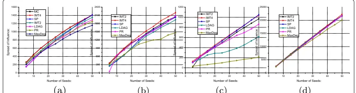
Figure 5 Simulation results of IMT whenTvaries in the range of [1,5] (spread of influence).(a)Hep, (b)Phy,(c)Amazon, and(d)Flixster.
in the range of [1, 5]. The simulation results are shown in Figure 5 and Table 2, in which MaxDeg and Random are considered as baselines. WhenT ≤ 4, the EIS is estimated by Algorithm 1; and whenT =5, it is estimated by Algorithm 2 with parameterr= 1, 000. Figure 5 shows the AIS of seed sets resulted by IMT, MaxDeg, and Random. First, the AIS of IMT in all the datasets is non-decreasing asTincreases. This agrees with our intuition in that increasing the number of hops brings more accurate EISE. Second, the increments of AIS are tiny when increasingT from 4 to 5, which implies that the seed quality of IMTT=4is as good as that of IMT5. From Figure 5, we also can get that the performance of IMTT=2is much better than that of IMTT=1for the first three data sets, and it is slightly worse than IMTT=4. In the ‘Flixster’ data set, all the algorithms perform similarly, except Random, which is always the worst one in all the experiments.
Consider now the running time performance. Table 2 shows the PRT of IMT, in which the file reading and writing time are not counted. WhenT ≤ 4, on the first three data sets, IMT is extremely fast, since the maximum out-degree in those data sets is not large. For instance, IMTT=4only requires less than 1 s to finish in ‘Hep’. In ‘Flixster’, IMT is fast whenT ≤2, and it is relatively slow whenT ≥4. WhenT=5, the PRT of IMT increases in certain degree for all the data sets. It is reasonable since in such a case, Algorithm 1 does not work, and Algorithm 2 is applied.
According to the first experiment, one notes that, in general, IMTT=4 is an efficient algorithm for seed selection. When the running time is of first priority or the data set is extremely large, IMTT=2is a good replacement.
In the second experiment, we compare IMTT=2and IMTT=4with the algorithms intro-duced in the ‘Algorithms’ section. The results are exhibited in Figure 6. Since MC is not scalable, its results are omitted for the last three data sets. As shown in Figure 6a, IMTT=4 and MC perform similarly in ‘Hep’. SP is about 2% lower than IMTT=4and MC in spread achieved when the number of seeds is 35, and its performance matches IMTT=4and MC when the number of seeds is greater or equal to 40. In the other three data sets, IMTT=4
Table 2 Running time performance (seconds)
Dataset Hep Phy Amazon Flixster
IMTT=1 0.14 0.28 0.37 1.32
IMTT=2 0.26 0.41 0.53 2.57
IMTT=3 0.46 0.92 1.01 30.54
IMTT=4 0.73 2.44 2.41 126.95
Figure 6 Simulation results of multiple methods on four datasets (spread of influence).(a)Hep, (b)Phy,(c)Amazon, and(d)Flixster.
is able to produce seed sets of the highest quality, and IMTT=2is also compatible with other algorithms in terms of AIS. In general, IMTT=4is the best one. In ‘Phy’, IMTT=4 outperforms SP by about 0% to 10%, and in ‘Amazon’ and ‘Flixster’, they perform similarly. IMTT=2outperforms PR and LDAG in ‘Hep’ and ‘Amazon’, and they perform similarly in ‘Phy’. In ‘Flixster’, all the methods perform well. More than 20K nodes can be activated by the seed set resulted by any algorithm in ‘Flixster’. It is probably because there are a lot of high-degree nodes in ‘Flixster’ (as shown in Table 1, the maximum degree node in ‘Flixster’ has 1,010 outgoing neighbors).
Although MC is able to produce high-quality seed sets, it is not scabble. In terms of PRT, IMTT=2is orders of magnitude faster than MC, and IMTT=4is also much faster than MC. According to the experiments, MC takes 8,532.6 s to finish in ‘Hep’. As shown in Table 2, the running time of IMTT=2and IMTT=4is only 0.26 and 0.73 s, respectively. Therefore, IMT is much more scalable than MC. In sum, IMT is better than other algorithms in terms of AIS except MC, and it is more suitable than MC for finding seed set in large social networks.
Finally, we would also like to evaluate the accuracy of our EISE algorithms. To do this, we compute the EIS for the most influential node in each data set by our EISE algorithms and by the SP algorithm, respectively. The results are compared with the exact solutions. Figure 7 shows the comparisons, in which ‘Ext’ denotes the exact EISTwhich is computed
by enumerating all the simple paths of length no more thanT. Our results exactly match the exact solutions whenT ≤ 4, which validates our conclusion in the ‘A deterministic algorithm’ section (EISE4is exact). For the case thatT =5, whenr=1, 000, the errors of EISE are about 1%, 2%, 0.1%, and 1% in the four data sets, whererdenotes the number of uniform random samples. Whenr=10, 000, the error is much lower. Compared with the
SP method with a pruning thresholdη, EISE is much more accurate in computing the EIS in data sets: ‘Hep’, ‘Phy’, and ‘Flixster’. In ‘Amazon’, the results of both EISE and SP match the exact solution. Note that in the second experiment, IMTT=4outperforms SP in ‘Hep’ and ‘phy’, and they perform similarly in ‘Amazon’. Thus, we can say that an accurate EISE algorithm is indeed important for solving the IM problem.
Conclusion
IM is a big topic in social network analysis. In this paper, we investigate efficient influence spread estimation for IM under the LT model. We analyze the problem both theoreti-cally and practitheoreti-cally. By adding a hop constraintT, we show that the influence estimation problem can be solved efficiently whenT is small, and it can be approximated well by uniform random sampling. Based on the two points, we develop a new algorithm called IMT for the LT model. The efficiency of IMT is demonstrated through simulations on four real-world social networks.
In future research, we plan to extend our work to other influence propagation models such as the IC model. Furthermore, we will study constraints under which the optimal solution for IM can be obtained.
Competing interests
The authors declare that they have no competing interests.
Authors’ contributions
ZL, LF, and KY formulated the problem and did the algorithm design and implementation. WW and BT contributed to the theoretical part of algorithm design and organized this research. All authors read and approved the final manuscript.
Acknowledgements
This research work was supported in part by the US National Science Foundation (NSF) under grants CNS 1016320 and CCF 0829993.
Received: 14 April 2014 Accepted: 22 May 2014
References
1. Domingos, P, Richardson, M: Mining the network value of customers. In: 2001 ACM SIGKDD Conference on Knowledge Discovery and Data Mining, pp. 57–66 San Francisco, CA, USA, (August 26-29, 2001)
2. Goldenberg, J, Libai, B, Muller, E: Using complex systems analysis to advance marketing theory development. Acad. Market. Sci. Rev.9(3), 1-18 (2001)
3. Goldenberg, J, Libai, B, Muller, E: Talk of the network: a complex systems look at the underlying process of word-of-mouth. Marketing Lett.12(3), 211–223 (2001)
4. Richardson, M, Domingos, P: Mining knowledge-sharing sites for viral marketing. In: the 2002 International Conference on Knowledge Discovery and Data Mining, pp. 61–70 Edmonton, AB, Canada, (July 23-25, 2002) 5. Kempe, D, Kleinberg, J, Tardos, É: Maximizing the spread of influence through a social network. In: The 2003 ACM
SIGKDD Conference on Knowledge Discovery and Data Mining, pp. 137–146 Washington, DC, USA, (August 24-27, 2003)
6. Ma, H, Yang, H, Lyu, MR, King, I: Mining social networks using heat diffusion processes for marketing candidates selection. In: The 2008 ACM Conference on Information and Knowledge Management, pp. 233–242 Napa Valley, CA, USA, (October 26-30, 2008)
7. Granovetter, M: Threshold models of collective behavior. Am. J. Sociol.83(6), 1420–1443 (1978) 8. Schelling, T: Micromotives and Macrobehavior. W.W. Norton, New York, USA, (1978)
9. Chen, W, Wang, Y, Yang, S: Efficient influence maximization in social networks. In: The 2009 ACM SIGKDD Conference on Knowledge Discovery and Data Mining, pp. 199–208 Paris, France, (June 28 - July 01, 2009)
10. Chen, W, Wang, C, Wang, Y: Scalable influence maximization for prevalent viral marketing in large-scale social networks. In: The 2010 ACM SIGKDD Conference on Knowledge Discovery and Data Mining, pp. 1029–1038 Washington DC, DC, USA, (July 25-28, 2010)
11. Chen, W, Yuan, Y, Zhang, L: Scalable influence maximization in social networks under the linear threshold model. In: The 2010 International Conference on Data Mining, pp. 88–97 Sydney, Australia, (December 14-17, 2010) 12. Narayanam, R, Narahari, Y: A Shapley value based approach to discover influential nodes in social networks. IEEE
Trans. Automation Sci. Eng.8(1), 130–147 (2011)
14. Jiang, Q, Song, G, Cong, G, Wang, Y, Si, W, Xie, K: Simulated annealing based in influence maximization in social networks. In: The 2011 AAAI Conference on Artificial Intelligence. San Francisco, CA, USA, (August 7-11, 2011) 15. Goyal, A, Lu, W, Lakshmanan, LVS: SIMPATH: an efficient algorithm for influence maximization under the linear
threshold model. In: The 2011 IEEE International Conference on Data Mining, pp. 211–220 Vancouver, Canada, (December 11-14, 2011)
16. Leskovec, J, Krause, A, Guestrin, C, Faloutsos, C, VanBriesen, J, Glance, NS: Cost-effective outbreak detection in networks. In: The 2007 ACM SIGKDD Conference on Knowledge Discovery and Data Mining, pp. 420–429 San Jose, CA, USA, (August 12-15, 2007)
17. Nemhauser, G, Wolsey, L, Fisher, M: An analysis of the approximations for maximizing submodular set functions. Math. Program.14(1978), 265–294 (1978)
18. Kimura, M, Saito, K, Nakano, R: Extracting influential nodes for information diffusion on social network. In: The 2007 AAAI Conference on Artificial Intelligence, pp. 1371–1376 Vancouver, British Columbia, (July 22-26, 2007)
19. Wang, Y, Cong, G, Song, G, Xie, K: Community-based greedy algorithm for mining top-kinfluential nodes in mobile social networks. In: The 2010 ACM SIGKDD Conference on Knowledge Discovery and Data Mining, pp. 1039–1048. Washington DC, DC, USA, (July 25-28, 2010)
20. Hoeffding, W: Probability inequalities for sums of bounded random variables. J. Am. Stat. Assoc.58(301), 13–30 (1963)
doi:10.1186/s40649-014-0002-3
Cite this article as:Luet al.:Efficient influence spread estimation for influence maximization under the linear threshold model.Computational Social Networks20141:2.
Submit your manuscript to a
journal and benefi t from:
7Convenient online submission 7Rigorous peer review
7Immediate publication on acceptance 7Open access: articles freely available online 7High visibility within the fi eld
7Retaining the copyright to your article


![Figure 5 Simulation results of IMT when T(b) varies in the range of [1,5] (spread of influence)](https://thumb-us.123doks.com/thumbv2/123dok_us/9608278.1943105/16.595.120.476.89.183/figure-simulation-results-imt-varies-range-spread-influence.webp)