The Thirty-Third AAAI Conference on Artificial Intelligence (AAAI-19)
Generalized Batch Normalization: Towards Accelerating Deep Neural Networks
Xiaoyong Yuan
∗ University of FloridaZheng Feng
∗ University of FloridaMatthew Norton
Naval Postgraduate SchoolXiaolin Li
University of FloridaAbstract
Utilizing recently introduced concepts from statistics and quantitative risk management, we present a general variant of Batch Normalization (BN) that offers accelerated conver-gence of Neural Network training compared to conventional BN. In general, we show that mean and standard deviation are not always the most appropriate choice for the centering and scaling procedure within the BN transformation, particularly if ReLU follows the normalization step. We present a Gen-eralized Batch Normalization (GBN) transformation, which
can utilize a variety of alternativedeviation measuresfor
scal-ing andstatisticsfor centering, choices which naturally arise
from the theory ofgeneralized deviation measuresand risk
theory in general. When used in conjunction with the ReLU non-linearity, the underlying risk theory suggests natural, ar-guably optimal choices for the deviation measure and statis-tic. Utilizing the suggested deviation measure and statistic, we show experimentally that training is accelerated more so than with conventional BN, often with improved error rate as well. Overall, we propose a more flexible BN transformation supported by a complimentary theoretical framework that can potentially guide design choices.
1
Introduction
Training a deep neural network has traditionally been a dif-ficult task. Issues such as the vanishing and exploding gradi-ent, see e.g., (Pascanu, Mikolov, and Bengio 2013), make the use of gradient based optimization techniques difficult from the perspective of stability and fast convergence. However, new, seemingly simple tools have emerged to help practi-tioners overcome common pitfalls of neural network train-ing. Two prominent examples are the use of Batch Normal-ization (BN) and Rectified Linear Units (ReLU).
Originally proposed by (Ioffe and Szegedy 2015), BN provides a simple transformation which incentivizes the ho-mogenization of neural network layer outputs, so as to have the same scale and mean, eliminating what is referred to as internal covariate shift. Intuitively, this allows the ‘signal’ flowing through the neural network to maintain a consis-tent center and scale, poconsis-tentially stabilizing gradients and the training procedure as a whole.
∗
Equal Contribution
Copyright c⃝2019, Association for the Advancement of Artificial
Intelligence (www.aaai.org). All rights reserved.
Consider a single layer of the network which first re-ceives output from the previous layer h and then applies an affine transformation to getx = W h+b, followed by an element-wise non-linearity to produce outputg(x)which is fed to the next layer. Let x = [x1, x2,· · ·, xn]T
de-note its individual components so that we can writeg(x) = [g(x1), g(x2), ..., g(xn)]T.
The BN transformation is based upon the following trans-formation on each dimensionjof the input,
ˆ
xj←
xj−E[xj] √
E[(xj−E[xj])2]
,
whereE[xj]and √
E[(xj−E[xj])2]are the mean and
stan-dard deviation of the random variable xj, which are
esti-mated during training with a batch of training examples. In this paper, we begin by asking the question: Are mean and standard deviation the right choice for every network architecture? This simple question leads us to the main con-tribution of this paper, which is the observation that batch normalization can naturally be generalized and improved by considering the general transformation,
ˆ
xj←
xj− S(xj) D(xj)
,
whereDis some measure ofdeviation, not necessarily the standard deviation, and whereS is astatisticwhich is not necessarily the mean. While arising from a specific set of axioms in risk theory, one can think ofDas a general mea-sure of the non-constancy ofxandSas a type of ’center.‘
We show that there exist many different choices for D
andSbesides standard deviation and mean, and that by for-mulating the batch normalization transformation with these alternatives one can accelerate neural network training com-pared to conventional BN and, in some settings, obtain im-proved predictive performance. Additionally, we show how the choice of DandS are driven not only by straightfor-ward intuition, but also by recently developed theoretical tools from statistics and risk theory. Specifically, the theory ofgeneralized deviation measuresprovides us with a wealth of choices fordeviation measureD, which includes standard deviation as a special case. In addition, for any choice ofD, there is a naturally correspondingstatisticS. Thus, choosing
Besides the simple observation that mean and standard deviation can be replaced by alternatives, our analysis is also driven by the observation that the appropriateness of the choice ofDandS is directly tied to the choice of non-linearity which follows the normalization transformation. We focus our analysis on the ReLU non-linearity from (Glo-rot, Bordes, and Bengio 2011) and (Nair and Hinton 2010), which has played a significant role in stabilizing and accel-erating neural network training (Krizhevsky, Sutskever, and Hinton 2012; Dahl, Sainath, and Hinton 2013). We show that mean and standard deviation are not natural choices for cen-tering and scaling if ReLU follows the normalization trans-formation. Risk theory and simple intuition suggest more natural choices. In fact, we see that one of these choices, the superquantile deviation, allows explicit control over the level of sparsity of activation’s; hypothesized to be an impor-tant property of ReLU (Glorot, Bordes, and Bengio 2011). While we focus on ReLU, this intuition can also be applied to any asymmetric non-linearity such as Leaky ReLU (Maas, Hannun, and Ng 2013), Exponential Linear Unit (Clevert, Unterthiner, and Hochreiter 2015), or any other arising from the ReLU family (e.g. (He et al. 2015)).
We demonstrate on MNIST, CIFAR-10, CIFAR-100, and SVHN datasets that the speed of convergence of stochastic gradient descent (SGD) can be increased by simply choos-ing a differentDandSand that, in some settings, we obtain improved predictive performance. Our experimental analy-sis also serves to support the intuition that ReLU paired with
D = √E[(x−E[x])2]andS = E[x]is a mismatch and
that asymmetric choices forDandS which are suggested by risk theory and intuition do, in fact, work better.
Although much further analysis is needed in this direc-tion, we show that the use of ReLU’s in tandem with BN can be tied directly to risk theory via a recently intro-duced concept called Buffered Probability of Exceedance (bPOE). Specifically, the use of normalization followed by a ReLU gives rise to what can be considered to be the tightest convex approximation to the 0 −1 loss. This is intriguing given the history of neural networks began with the concept of0−1loss (indicator function) neural output which were then approximated with the sigmoid transforma-tion as a differentiable surrogate (see e.g. (Rosenblatt 1958; McCulloch and Pitts 1943)).
2
Batch Normalization
The BN transformation is based upon the following trans-formation on each dimensionjof the input,
ˆ
xj←
xj−µj
√
σ2
j+ϵ
,
whereσj andµj are the empirical standard deviation and
mean of the random variablexj, which are estimated during
training with a batch of training examples. Throughout this paper, we will viewxas a random vector which is observed empirically via the training batches. Thus, during training,
µj = |B1|
∑|B| i=1x
(i)
j with|B|denoting the size of the
train-ing batch.
The BN procedure follows the actual normalization with the following linear transformation, whereγj, βjare
param-eters which will be tuned during training,
γjxˆj+βj.
The BN procedure is then followed by the final non-linear transformationg(γjxˆj+βj). Why is this linear
transforma-tion needed? As noted by (Ioffe and Szegedy 2015), the BN transformation may not be appropriate or work well in con-junction with the non-linear transformationg that follows. Thus, the authors introduced a way to adjust the BN trans-formation if necessary. However, there is no guarantee that training will find the right linear transformation and be able to properly counteract a poor choice of scale and center. In some sense, this is why it is argued in (Mishkin and Matas 2015) that proper initialization is all that is needed. Assum-ing that the centerAssum-ing and scalAssum-ing are not correct, which is to say that the trainable linear transformation is necessary to adjust the center and scale, then BN can be loosley viewed as a type of data dependent initialization strategy. In this sense, the additional linear transformation can be used within our proposed scheme in exactly the same way, but with more control over the initialization where one would hope to se-lect a more appropriate data-dependent centering and scaling factor.
Cases where the standard BN may not work well in conjunction with the non-linearity g can be easily illus-trated, particularly if g is the ReLU non-linearity. Con-sider a set of outputs {x1,· · · , xN} from a network layer
which have mean zero, i.e., N1 ∑N
i=1xi = 0, with
order-ing x1 < · · · < xk < 0 < xk+1 < · · · < xN.
As-sume that we are then going to divide by some normaliza-tion factor, such as standard devianormaliza-tion, and then feed these values into a ReLU non-linearity max{0, xi}. The ReLU
non-linearity will map points x1,· · ·, xk to zero.
Consid-ering this fact, does it make sense to first divide the whole set of N points by the standard deviation? Intuitively, it would make more sense to divide by the variance of only the set of points{xk+1,· · · , xN}. The variation of the set
of points {x1,· · ·, xk} is irrelevant given the fact that a
ReLU will follow, sending all of these points to zero. This consideration is particularly important if the conditional dis-tributions {x1,· · · , xk} and {xk+1,· · ·, xN} exhibit very
different scales and variation. In this case, it may be more appropriate to use a one-sided measure of deviationD for the normalization step such as the Right Semi-Deviation (RSD) N1 ∑N
i=1max{0, xi}. Furthermore, a similar
argu-ment can be applied to the centering operation. Assume, for instance, that the distribution{x1,· · ·, xN}is heavy-tailed,
with{x1,· · ·, xN−1}having mean zero and variance 1, but
with xN = 100. The mean of all N points will be very
large, and centering the data via mean subtraction will yield
xN −µas the only term with value larger than zero. Thus,
the application of the ReLU will leave only one sample as having non-zero value (and gradient), with much of the valu-able learning signal lost because of poor choice of centering statisticS.
ad-just the normalization with the affine transformation (or at least reducing the amount by which it would need to be adjusted), offering accelerated convergence. Generalizations and variants of BN have been proposed before. For example, Klambauer et al. (2017) proposed a self-normalizing net-work layer, but is limited to standard feed-forward architec-tures. Ba, Kiros, and Hinton (2016) altered BN to work with recurrent neural networks. Mishkin and Matas (2015) argue that BN is simply another way to perform initialization, thus proposing initialization methods that produce similar ef-fects. The idea of BN was altered to weight normalization by reparameterizing the weights (Salimans and Kingma 2016; Chunjie, Qiang, and others 2017). Our proposed approach, while relying on simple principles, is grounded in a broader theory and maintains all important flexibility of conventional BN.
3
Asymmetric Deviation Measures in Risk
Theory
As alluded to in the introduction, it is easy to question the use of variance as the scale normalizing factor if it is fol-lowed by the ReLU transformation. This gives rise to the ob-vious question: What other options do we have that may be more appropriate? We find, in general, that risk theory pro-vides us with an entire class of generalized deviation mea-sures to choose from. In this section, we briefly introduce risk theory before discussing generalized deviation mea-sures in Section 4 where we introduce the GBN transforma-tion and show that generalized deviatransforma-tion measures provide us with an array of alternatives to mean and standard devia-tion.
Over the past 25 years, risk management theory has played a crucial role in the development of fundamental statistical concepts that not only measure risk (Artzner et al. 1999; F¨ollmer and Schied 2002; Szeg¨o 2002), but have proven fundamental to statistical theory and optimization under uncertainty. A full review of risk theory is beyond the scope of this paper, but a simple example in the context of financial engineering can be used to illustrate. Consider an investment which will yield a loss ofx, withxbeing a ran-dom monetary loss. Assume we knew the distribution ofx, and we were to ask: Howriskyis this investment? How can we measureriskto compare it against other investmentsy? An obvious choice would be to look at the expected loss
E[x]. However, this may be inappropriate, as investor ob-jectives (or distribution of x) may be highly asymmetric. It may be more appropriate to measure risk with an asym-metric quantity. One example would be to use the
quan-tile qα(x) = min{z|P(x ≤ z) ≥ α}, where α ∈ [0,1]
is a probability level. Its inverse, called Probability of Ex-ceedance (POE), given byP(x > z)wherez∈ Ris some
known threshold, may also be desirable if some thresholdz
is known and exceeding such a threshold is undesirable. One of the primary drivers of risk theory, however, has been the need to quantify risk in such a way that optimiza-tion can take place (e.g. finding the portfolio with minimal risk). The quantile, also called the Value-at-Risk, and POE are numerically troublesome in this context. Specifically,
these functions often prove to be non-convex and discontin-uous, essentially reducing to sums of indicator (0−1loss) functions. From this difficulty, more amenable alternatives have arisen.
Two popular alternatives that are relevant to our discus-sion are the superquantile and Buffered Probability of Ex-ceedance (bPOE) (Rockafellar and Uryasev 2000; Rockafel-lar and Uryasev 2002; Acerbi and Tasche 2002; Mafusalov and Uryasev 2015). The superquantile is a measure of un-certainty similar to the quantile, but with superior mathe-matical properties. Formally, the superquantile, also called Conditional Value-at-Risk (CVaR) in the financial engineer-ing literature, for a continuously distributedxis defined as
¯
qα(x) =E[x|x > qα(x)].
For general distributions, the superquantile can be defined by the following formula,
¯
qα(x) = min
γ γ+
E[x−γ]+
1−α , (1)
where[·]+= max{·,0}.
Similar toqα(x), the superquantile can be used to assess
the tail of the distribution. The superquantile, though, is far easier to handle in optimization contexts. It also has the im-portant property that it considers the magnitude of events within the tail. Therefore, in situations where a distribution may have a heavy tail, the superquantile accounts for mag-nitudes of low-probability large-loss tail events while the quantile does not account for this information.
bPOE is the inverse of the superquantile. In other words, bPOE calculates one minus the probability level at which the superquantile equals a specified thresholdz. It is calculated by the formula
¯
pz(x) = min
a≥0E[a(x−z) + 1]
+= min
γ<z
E[x−γ]+
z−γ ,
where[·]+= max{·,0}.In addition, we have the following formula which will be important for our case. Assuming that
¯
pz(x) = 1−α, we have that
¯
pz(x) =
E[x−qα(x)]+
¯
qα(x)−qα(x)
.
Roughly speaking, bPOE calculates the proportion of worst case outcomes which average toz.
As it relates to POE, bPOE can be viewed as an opti-mal convex approximation. More specifically, among law-invariant functions of x, p¯z(x) is the minimal (tightest)
4
Generalized Batch Normalization
In this paper, we define Generalized Batch Normalization (GBN) to be identical to conventional BN but with stan-dard deviation replaced by a more general deviation mea-sureD(x)and the mean replaced by a corresponding statis-ticS(x). In other words, we have the transformation,ˆ
xj←
xj− S(xj) D(xj)
.
Here, each choice of D is naturally paired with some S, which we discuss in the following section. In Section 5, we implement a suite of these new measures and test them on the MNIST, CIFAR-10, CIFAR-100, and SVHN datasets, showing that convergence can be accelerated, and sometime accuracy improved, by use of different deviation measures and statistics.
4.1
Generalized Deviation Measures and
Statistics
In (Rockafellar, Uryasev, and Zabarankin 2006), the con-cept of a generalized deviation measure was introduced to broaden the statistical view ofdeviation beyond the single case of standard deviation, specifically for use in quantita-tive risk analysis. These deviation measures follow a very general set of axioms which we will not delve into here. However, some examples can be found in Table 1, and they can be understood intuitively as follows: Deviation measures quantify thenon-constancyof a random variable. As seen in Table 1, standard deviation is only one of many possibilities, such as the asymmetric deviation measures RSD and SQD
withα > 0. These measures of deviation look at the
vari-ation only in theright-tailof the distribution ofx. It’s easy to see how this type of asymmetric measure would be of in-terest in finance, where it may be important to analyze the variation of only the largest losses within theright-tail.
The theory of generalized deviation measures is also com-plemented by the recently introduced theory of the Risk Quadrangle. Utilizing functional relationships that are be-yond the scope of this paper, (Rockafellar and Uryasev 2013) shows that measures of deviation are intimately re-lated to similar measures of risk, regret, and error. Further-more, associated with any measure of deviation is a unique
statistic. In short, however, without getting into too much detail, one can think of the statistic as a type of ‘center.’ In Table 1, we see how this intuition plays out, with the corre-sponding statistics listed in the right column. For SD, MAD, and RSD, we see thatS(x)is simply the expectation. How-ever, for SQD withα= .5, we see thatS(x) = q.5(x)the
median, certainly a different notion of the ‘center.’ Further-more, we see that for RBD, the statistic is the center of the range. However, for SQD it is important to notice that we can achieve very different statistics by movingα, which gives us different quantiles.
4.2
Choosing
D
or
S
: General Intuition
Now that we are given more options for deviation measures and statistics, we can begin to think about the benefits and drawbacks of each within the neural network architecture
and the GBN transformation. Utilizing standard deviation seems like an intuitive choice. However, this depends heav-ily on the shape of the (empirical) distribution ofx. If the distribution is relatively symmetric, then standard deviation will be indicative of the overall scale and the mean will be indicative of the ‘center’. Similarly, this may hold true if the distribution does not have heavy tails or outliers on one side or the other. However, if the distribution ofxhas e.g. heavy tails, is highly asymmetric, has outliers, or is multimodal; then the mean may be a poor choice for the ‘center’ and the deviation of values to the right of the mean may be dra-matically different than the deviation of values to the left of the mean. In this case, a quantile may be a more appropri-ate notion of the ‘center.’ Choosing, for example, the median instead of the mean assures that we are truly ‘centering’ the data, with half of the points on the ‘left’ and half on the ‘right.’
Even if the distribution ofxis not asymmetric or heavy tailed, the choice of center is particularly important if nor-malization is followed by the ReLU activation. Specifically, the choice of center controls the sparsity of activation’s pro-duced by the ReLU, since any elements left-of-center will be sent to zero. ReLU induced sparsity has been hypothe-sized as critical to its success (Glorot, Bordes, and Bengio 2011). In this case, the quantile is a natural choice for cen-ter that provides precise control over such sparsity. If the normalization centers w.r.t. the quantile atα, exactlyα%of activation’s across the batch will have zero value.
Driving our intuition from the beginning was the idea that the non-linearity, deviation measure, and statistic should be chosen in tandem. As mentioned in Section 2, the pairing of ReLU with typical BN (i.e. standard deviation and mean normalization) does not seem appropriate given the fact that standard deviation is symmetric while ReLU is asymmetric. Thus, in light of Section 2, we find that asymmetric deviation measures are more appropriate such as RSD or SQD for any
α > 0. In Section 5, we see this intuition confirmed, with
RSD and SQD outperforming SD in terms of convergence rate and, often times, test error. Although not explored in our experiments, this intuition applies to any asymmetric non-linearity such as the Leaky ReLU (Maas, Hannun, and Ng 2013), Exponential Linear Unit (Clevert, Unterthiner, and Hochreiter 2015), or any other arising from the ReLU family (e.g. (He et al. 2015)).
4.3
An Optimal Choice
Beyond this simple intuition, we can utilize connections to risk theory to provide evidence that the ReLU should be used in tandem with an asymmetric deviation measure. Specifi-cally, we show that the use of SQD and RSD followed by ReLU is approximately equivalent to a probabilistic trans-formation which mimics an optimal quasiconvex approxi-mation to the0−1(indicator) loss function.
Deviation MeasureD(x) StatisticS(x)
Standard Deviation (SD) √E[(x−E[x])2] E[x]
Mean Absolute Deviation (MAD) E[|x−E[x]|] E[x]
Right-Semi-Deviation (RSD) E[x−E[x]]+ E[x]
Superquantile Deviations (SQD) forα∈(0,1) q¯α(x−E[x]) qα(x)
Range-Based Deviation (RBD) supx−infx 1
2(supx+ infx)
Worst-Case Deviation (WCD) supx−E[x] supx
Table 1: Examples of deviation measures and their corresponding statistics.[x]+= max{0, x}
Now, for the GBN transformation let us choose SQD devi-ation measureD(xj) = ¯qα(xj−µj)whereαis chosen so
thatqα(xj) = µj, meaning that we are choosing the
prob-ability level on which the mean sits. This gives us the fol-lowing transformation, where the superscript denotes theith
sample from a batch:
ˆ
x(ji)←
[
x(ji)−qα(xj)
¯
qα(xj)−qα(xj) ]+
.
This can be re-written as,
ˆ
x(ji)←
[
x(ji)−µj
E[xj−µj|xj > µj] ]+
.
One will immediately notice that this is almost identical to a conventional BN transformation followed by ReLU with the only difference being that we are dividing by a one-sided semi-deviation rather than the two-one-sided standard de-viation. One will notice, however, the following connection to bPOE:
¯
pz(xj) =E
[ x
j−qα(xj)
¯
qα(xj)−qα(xj) ]+
for thresholdz = ¯qα(xj). Thus, we see that the
combina-tion of GBN and ReLU yields a transformacombina-tion based upon bPOE. If also divided by sample size N, each individual
samplex(ji)will yield output N1 [
x(ji)−qα(xj)
¯
qα(xj)−qα(xj)
]+
∈ (0,1)
with the sum,
1
N
[
x(ji)−qα(xj)
¯
qα(xj)−qα(xj) ]+
= ¯pˆz(xj),
wherep¯ˆz(xj)simply denotes the empirical bPOE calculated
from a sample. This means that the overall output distribu-tion will consist of values in the range[0,1]with non-zero items being those that are in the bPOE-tail of the empirical distribution ofxj.
Thus, by combining GBN and ReLU we are effectively performing a probabilistic transformation, with the transfor-mation mimicking the optimal quasiconvex approxitransfor-mation to the0−1loss.
5
Experimental Evaluation
Overall, the first goal of our experiments is to demonstrate the obvious: All other things being equal, different normal-ization methods (i.e. different choices for deviation measure
and statistic) lead to different network properties. We then explore the specifics of these changes. First, we show that convergence rate and stability of NN training via SGD can often be improved by utilizing alternative deviation mea-sures. Improvement is measured relative to conventional BN, which uses mean and standard deviation as its statistic and deviation measure. Overall, we find that SQD, MAD, and RSD often lead to increased convergence rates and, sometimes, increased stability in terms of smoothly decreas-ing test error durdecreas-ing SGD. Second, we see that these alterna-tive choices often lead to testing error that is nearly as good as, or better, than that achieved by standard BN.
For all experiments, GBN is implemented in exactly the same manner as standard BN, only with mean and variance replaced by generalizedS andDwithin the batch normal-ization transformation. This includes appropriate inclusion of the chosen deviation measure and statistic within the gra-dient calculation as well as the batch-based estimation of
D(xj)andS(xj)during training and population-based
es-timation for inference. This also includes the additional lin-ear transformation which typically follows the normaliza-tion step, before applicanormaliza-tion of non-linearity. See (Ioffe and Szegedy 2015) for specifics.
We performed experiments on MNIST, CIFAR-10, CIFAR-100, and SVHN datasets. We compared the perfor-mance of GBN transformations with 7 different deviation measures and statistics, including the conventional mean and standard deviation. As indicated in Table 1, we utilized standard SD along with MAD, RSD, RBD, and SQD with
α = .25, .5, and.75 which we denote by SQD1, SQD2, and SQD3 respectively. We omit WCD since centering w.r.t.
supxis obviously a poor choice when paired with ReLU. Subtractingsupxwould make all points less than or equal to zero and the ReLU would send them all then to zero, pro-ducing an untrainable network without activations.
5.1
MNIST
(a) Before the standard BN (b) After the standard BN
(c) Before the GBN with SQD1 (d) After the GBN with SQD1
0 1 2 3 4 5 0.0
0.2 0.4 0.6
0.8 SQD1SD
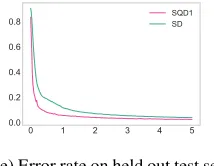
(e) Error rate on held out test set
Figure 1: (a, b) The distribution evolution of standard BN on a selected feature along with the iteration steps. (c, d) The same figure over the GBD with SQD1 deviation measure. (e) The error rate of two settings on the held out test set. GBN with SQD1 help the network converges faster and also achieves better error rate that standard BN.
is performed on standard BN and GBN with deviation mea-sure SQD1, which has statistic equal to theα =.25 quan-tile. We choose to observe one feature pixel of the second convolutional layer’s feature map. Figure 1(a,b) shows this feature’s distribution density before and after standard BN. Figure 1(c,d) shows the same feature’s distribution density before and after applying GBN with SQD1. All the distribu-tions before batch normalization exhibit significant change in terms of mean and variance. Both of the two normaliza-tion approaches removed the covariate shift effect and out-put a stabilized distribution over time. And after GBN with the deviation measure of SQD1, most of the values appear larger than 0 compared to the symmetric distribution of stan-dard BN having the mean of 0. As one would expect, cen-tering w.r.t. theα = .25quantile forcesα%of the activa-tions to be less than zero before applying the non-linearity. In Figure 1(e), this consistent asymmetric distribution of the GBN’s output helps it achieve faster convergence rate and better error rate compared to the standard BN.
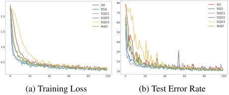
GBN performance on MNIST To compare the perfor-mance of various deviation measures and statistics on MNIST, we use the same experimental setting of neural net-work above with vanilla SGD as the optimizer, with learn-ing rate equal to.01, and batch size equal to 1000. Figure 2 shows the error rate of 6 different choices for deviation
mea-0 2 4 6 8 10
0.0 0.5 1.0 1.5 2.0
SD RSD SQD1 SQD2 SQD3 MAD
(a) Training Loss
0 2 4 6 8 10
0 20 40 60
80 SDRSD
SQD1 SQD2 SQD3 MAD
(b) Test Error Rate(%)
Figure 2: Performance comparison of the MNIST classifica-tion with LeNet. X-axis: Number of epochs; Y-axis: Train-ing loss/Test error rate.
sure and statistic. All settings are evaluated on the training loss and test error rate. We see that GBN with SQD1, RSD, SQD2, and MAD all perform better than standard BN in terms of converge rate and test error rate. And GBN with deviation measures of SQD1 and RSD converge remarkably faster than others.
5.2
CIFAR-10, CIFAR-100, and SVHN
We compare the performance and convergence rate on the CIFAR-10, CIFAR-100, and Street View House Numbers (SVHN) datasets. The CIFAR-10 and CIFAR-100 dataset consist of 60,000 tiny color images (32x32) with 10 and 100 classes respectively for image recognition task (Krizhevsky and Hinton 2009). The SVHN Dataset consists of Google Street View images with 10 house digit classes (Netzer et al. 2011).
We trained LeNet networks on the CIFAR-10 (200 epochs) and the SVHN (200 epochs) datasets. The setting is set similar to that used with MNIST dataset: SGD with learning rate 0.1 and 0.01, batch size 1024. Figure 3 and Fig-ure 4 illustrate the performance comparison of six different choices of deviation measure on the CIFAR-10 and SVHN datasets respectively.
We also train a ResNet architecture with 20 layers (ex-actly the same architecture and settings used in (He et al. 2015)) for 200 epochs on the CIFAR-10 and CIFAR-100 dataset. We trained the ResNet with and without data aug-mentation (i.e., random crop and random horizontal flip). For the CIFAR-10 dataset, we observe that with data aug-mentation, the proposed methods achieve the similar per-formance as standard BN. However, if we do not augment data (less symmetric distribution), both RSD and MAD per-form better than standard BN (Figure 5). For the CIFAR-100 dataset, even with data augmentation, RSD and MAN out-perform standard BN (Figure 6).
Dataset Architecture Learning Rate Batch Size SD MAD RSD RBD SQD1 SQD2 SQD3
CIFAR-10 LeNet 0.1 256 30.73 29.70 30.04 30.38 33.29 29.53 29.07
CIFAR-10 LeNet 0.1 1024 29.31 28.58 28.85 31.05 33.33 28.63 28.03
CIFAR-10 LeNet 0.1 2048 28.96 29.32 27.51 36.28 39.94 28.79 29.18
CIFAR-10 LeNet 0.01 256 29.69 29.03 29.90 33.32 29.99 27.96 27.36
CIFAR-10 LeNet 0.01 1024 28.29 28.37 29.44 47.51 30.62 29.33 30.97
CIFAR-10 LeNet 0.01 2048 31.64 30.53 30.81 57.08 32.45 31.35 37.26
CIFAR-10 ResNet20 0.1 1024 29.67 29.33 30.55 20.49 23.64 24.86 24.99
CIFAR-10 ResNet20 0.01 1024 34.57 33.59 35.52 47.17 32.20 32.02 47.89
SVHN LeNet 0.1 1024 10.68 10.17 10.91 12.17 80.41 10.60 10.08
SVHN LeNet 0.1 2048 10.46 10.18 10.57 13.58 22.03 10.68 9.75
SVHN LeNet 0.01 1024 10.83 10.46 10.30 20.62 11.62 10.87 11.29
SVHN LeNet 0.01 2048 12.60 11.74 11.22 43.04 11.99 11.83 12.80
Table 2: Performance Comparison of Test Error Rate (%) on the CIFAR-10 and SVHN datasets.
0 20 40 60 80 100 120 140 0.50
0.75 1.00 1.25 1.50 1.75 2.00
2.25 SDRSD SQD1 SQD2 SQD3 MAD
(a) Training Loss
0 20 40 60 80 100 120 140 30
40 50 60 70 80
SD RSD SQD1 SQD2 SQD3 MAD
(b) Test Error Rate
Figure 3: Performance comparison on the CIFAR-10 dataset using LeNet. X-axis: Number of epochs; Y-axis: Training loss/Test error rate (%).
0 20 40 60 80 100 0.5
1.0 1.5 2.0
SD RSD SQD1 SQD2 SQD3 MAD
(a) Training Loss
0 20 40 60 80 100 10
20 30 40 50 60 70
80 SD
RSD SQD1 SQD2 SQD3 MAD
(b) Test Error Rate
Figure 4: Performance comparison on the SVHN dataset. X-axis: Number of epochs; Y-X-axis: Training loss/Test error rate (%).
5.3
Discussion
When choosingSandD, it is important to consider their es-timation properties. For example, it is well-known that em-pirical estimates of the mean are more stable, and converge more quickly to the true mean, than empirical estimates of the superquantile. This also applies to SD and one-sided de-viation measures like RSD. Clearly, since only one side of the distribution is involved, more samples will be needed for accurate, low variance estimation of asymmetric (one-sided) deviation measures or statistics. Compared with small batch size, we observe that training with large batch size improves the convergence rate. However, this small-batch degradation
0 25 50 75 100 125 150 175 200 1
2 3 4
SD RSD SQD1 SQD2 SQD3 MAD
(a) Training Loss
0 25 50 75 100 125 150 175 200 40
50 60 70 80
90 SD
RSD SQD1 SQD2 SQD3 MAD
(b) Test Error Rate
Figure 5: Performance comparison on the CIFAR-10 dataset using ResNet20. X-axis: Number of epochs; Y-axis: Train-ing loss/Test error rate (%).
0 25 50 75 100 125 150 175 200 2
4 6 8
10 SDRSD
SQD1 RBD SQD3 MAD
(a) Training Loss
0 25 50 75 100 125 150 175 200 40
50 60 70 80 90
100 SD
RSD SQD1 RBD SQD3 MAD
(b) Test Error Rate
Figure 6: Performance comparison on the CIFAR-100 dataset using ResNet20. X-axis: Number of epochs; Y-axis: Training loss/Test error rate (%).
is not a new consideration and has been observed with stan-dard BN. (Ioffe 2017) discusses this issue and shows that there do exist techniques to help alleviate this affect for BN. Although we leave this discussion to future work, it would seem straightforward to apply the same techniques to GBN in general.
6
Conclusion
are many other natural choices for the scaling and center-ing factors which we pose as general deviation measures and statistics. We also show that conventional normalization is not optimal if followed by the ReLU non-linearity and we provide alternatives that are justified both intuitively and theoretically, showing also that these new methods increase convergence speed experimentally.
7
Acknowledgement
The authors would like to thank anonymous reviewers whose suggestions help improve the quality of the paper. This research was supported in part by National Science Foundation (CNS-1624782, CNS-1747783), National Insti-tutes of Health (R01-GM110240), and Industrial Members of NSF Center for Big Learning (CBL).
References
Acerbi, C., and Tasche, D. 2002. On the coherence of expected shortfall.Journal of Banking & Finance26(7):1487–1503. Artzner, P.; Delbaen, F.; Eber, J.-M.; and Heath, D. 1999. Co-herent measures of risk.Mathematical finance9(3):203–228. Ba, J. L.; Kiros, J. R.; and Hinton, G. E. 2016. Layer normal-ization.arXiv preprint arXiv:1607.06450.
Chow, Y., and Ghavamzadeh, M. 2014. Algorithms for cvar optimization in mdps. InNIPS, 3509–3517.
Chunjie, L.; Qiang, Y.; et al. 2017. Cosine normalization: Us-ing cosine similarity instead of dot product in neural networks.
arXiv preprint arXiv:1702.05870.
Clevert, D.-A.; Unterthiner, T.; and Hochreiter, S. 2015. Fast and accurate deep network learning by exponential linear units (elus).arXiv preprint arXiv:1511.07289.
Dahl, G. E.; Sainath, T. N.; and Hinton, G. E. 2013. Improving deep neural networks for lvcsr using rectified linear units and dropout. InICASSP, 8609–8613. IEEE.
F¨ollmer, H., and Schied, A. 2002. Convex measures of risk and trading constraints.Finance and stochastics6(4):429–447. Galichet, N.; Sebag, M.; and Teytaud, O. 2013. Exploration vs exploitation vs safety: Risk-aware multi-armed bandits. In
Asian Conference on Machine Learning, 245–260.
Glorot, X.; Bordes, A.; and Bengio, Y. 2011. Deep sparse rectifier neural networks. InProceedings of the Fourteenth In-ternational Conference on Artificial Intelligence and Statistics, 315–323.
Gotoh, J.-y., and Uryasev, S. 2017. Support vector machines based on convex risk functions and general norms. Annals of Operations Research249(1-2):301–328.
He, K.; Zhang, X.; Ren, S.; and Sun, J. 2015. Delving deep into rectifiers: Surpassing human-level performance on ima-genet classification. InICCV, 1026–1034.
Ioffe, S., and Szegedy, C. 2015. Batch normalization: Acceler-ating deep network training by reducing internal covariate shift. InICML, 448–456.
Ioffe, S. 2017. Batch renormalization: Towards reducing mini-batch dependence in mini-batch-normalized models. InNIPS, 1942– 1950.
Klambauer, G.; Unterthiner, T.; Mayr, A.; and Hochreiter, S. 2017. Self-normalizing neural networks. InNIPS, 972–981.
Krizhevsky, A., and Hinton, G. 2009. Learning multiple layers of features from tiny images. Technical report, University of Toronto.
Krizhevsky, A.; Sutskever, I.; and Hinton, G. E. 2012. Im-agenet classification with deep convolutional neural networks. InNIPS, 1097–1105.
LeCun, Y.; Bottou, L.; Bengio, Y.; and Haffner, P. 1998. Gradient-based learning applied to document recognition. Pro-ceedings of the IEEE86(11):2278–2324.
Maas, A. L.; Hannun, A. Y.; and Ng, A. Y. 2013. Rectifier non-linearities improve neural network acoustic models. InProc. icml, volume 30, 3.
Mafusalov, A., and Uryasev, S. 2015. Buffered probability of exceedance: Mathematical properties and optimization al-gorithms. Research Report 2014-1, ISE Dept., University of Florida.
McCulloch, W. S., and Pitts, W. 1943. A logical calculus of the ideas immanent in nervous activity. The bulletin of mathemati-cal biophysics5(4):115–133.
Mishkin, D., and Matas, J. 2015. All you need is a good init.
arXiv preprint arXiv:1511.06422.
Nair, V., and Hinton, G. E. 2010. Rectified linear units improve restricted boltzmann machines. InICML, 807–814.
Netzer, Y.; Wang, T.; Coates, A.; Bissacco, A.; Wu, B.; and Ng, A. Y. 2011. Reading digits in natural images with unsuper-vised feature learning. InNIPS workshop on deep learning and unsupervised feature learning, volume 2011, 5.
Norton, M.; Mafusalov, A.; and Uryasev, S. 2017. Soft margin support vector classification as buffered probability minimiza-tion.JMLR18(1):2285–2327.
Pascanu, R.; Mikolov, T.; and Bengio, Y. 2013. On the difficulty of training recurrent neural networks. InICML.
Rockafellar, R., and Uryasev, S. 2000. Optimization of condi-tional value-at-risk. The Journal of Risk, Vol. 2, No. 3, 2000, 21-41.
Rockafellar, R. T., and Uryasev, S. 2002. Conditional value-at-risk for general loss distributions.Journal of banking & finance
26(7):1443–1471.
Rockafellar, R. T., and Uryasev, S. 2013. The fundamental risk quadrangle in risk management, optimization and statistical estimation. Surveys in Operations Research and Management Science18(1):33–53.
Rockafellar, R. T.; Uryasev, S.; and Zabarankin, M. 2006. Gen-eralized deviations in risk analysis. Finance and Stochastics
10(1):51–74.
Rosenblatt, F. 1958. The perceptron: A probabilistic model for information storage and organization in the brain. Psychologi-cal review65(6):386.
Salimans, T., and Kingma, D. P. 2016. Weight normalization: A simple reparameterization to accelerate training of deep neural networks. InNIPS, 901–909.
Szeg¨o, G. 2002. Measures of risk. Journal of Banking &
Finance26(7):1253–1272.
![Table 1: Examples of deviation measures and their corresponding statistics.[x]+ = max{0, x}](https://thumb-us.123doks.com/thumbv2/123dok_us/9668728.1949655/5.612.113.505.53.135/table-examples-deviation-measures-corresponding-statistics-x-max.webp)