An upwind least square formulation
for free surfaces calculation of viscoplastic
steady‑state metal forming problems
Ugo Ripert
1*, Lionel Fourment
2and Jean‑Loup Chenot
1Background
One or two decades ago, when computers resources were much lower, steady-state for-mulations have attracted considerable interest in the field of material forming simulation More precisely in the metal forming field, it was extensively applied for rolling processes. Early simulations were done for thick plates [1] and simple shape rolling [2]. They were extended to seamless tube rolling [3, 4] and complicated shape rolling [5] before being applied to more complex material behavior [6] and to rolling stand deformation [7].
Abstract
Despite using very large parallel computers, numerical simulation of some forming processes such as multi‑pass rolling, extrusion or wire drawing, need long computa‑ tion time due to the very large number of time steps required to model the steady regime of the process. The direct calculation of the steady‑state, whenever possible, allows reducing by 10–20 the computational effort. However, removing time from the equations introduces another unknown, the steady final shape of the domain. Among possible ways to solve this coupled multi‑fields problem, this paper selects a staggered fixed‑point algorithm that alternates computation of mechanical fields on a prescribed domain shape with corrections of the domain shape derived from the velocity field and the stationary condition v.n= 0. It focuses on the resolution of the second step in the frame of unstructured 3D meshes, parallel computing with domain partitioning, and complex shapes with strong contact restraints. To insure these constraints a global finite elements formulation is used. The weak formulation based on a Galerkin method of the v.n = 0 equation is found to diverge in severe tests cases. The least squares formulation experiences problems in the presence of contact restraints, upwinding being shown necessary. A new upwind least squares formulation is proposed and evaluated first on analytical solutions. Contact being a key issue in forming processes, and even more with steady formulations, a special emphasis is given to the coupling of contact equations between the two problems of the staggered algorithm, the thermo‑mechanical and free surface problems. The new formulation and algorithm is finally applied to two complex actual metal forming problems of rolling. Its accuracy and robustness with respect to the shape initialization of the staggered algorithm is discussed, and its efficiency is compared to non‑steady simulations.
Keywords: Steady‑state, Free surface, Least square formulation, Upwind shift, SUPG, Contact, Metal forming, Rolling, Finite elements
Open Access
© 2015 Ripert et al. This article is distributed under the terms of the Creative Commons Attribution 4.0 International License (http:// creativecommons.org/licenses/by/4.0/), which permits unrestricted use, distribution, and reproduction in any medium, provided you give appropriate credit to the original author(s) and the source, provide a link to the Creative Commons license, and indicate if changes were made.
RESEARCH ARTICLE
*Correspondence: [email protected]
1 Transvalor, 694 avenue
Maurice Donat Parc de Haute Technologie, 06250 Mougins, France
This was often justified by the fact that it was not possible to simulate the unsteady problem in all its complexity at that time. Nowadays, few publications using these meth-ods can be found in the open literature, either because software codes are now quite mature and currently used in R&D [8] or because present computer resources make full, time-dependent simulations possible. However, some metal forming simulations still end up with computational times (several weeks or months) that are much too large for prac-tical use by the engineer. This mainly occurs wherever resolution requires a very large number of time steps—such problems cannot therefore be accelerated by a larger number of processors. Moreover, as the efficiency of computing processors does not increase as it used to, perspectives to reduce the computational time of these problems are shrinking. Therefore, for appropriate problems, the steady-state formulations arise again as a way to reduce the computational times by one to two orders of magnitude. The work presented in this paper is carried out in the frame of material forming in order to adapt and general-ize some steady-state formulations to today’s numerical methods (unstructured meshes and parallel computations) and problems complexity (geometries and robustness).
Semi-continuous metal forming processes such as rolling or wire drawing can be sim-ulated by the same numerical methods that are utilized for more conventional processes, like an incremental formulation within a Lagrangian framework [9]. Such an approach is indispensable in studies of intrinsically transient phenomena such as end geometry, edg-ing strategies, crocodiledg-ing, twistedg-ing… However, when it comes to long products, most of the process can be regarded as stationary, and the forming of product ends is of sec-ondary interest. In order to reach this stationary regime by passing the initial transient regime, very long sections of the product must be considered and consequently very large finite element meshes. In addition, the time steps must be small enough to properly capture the local contact phenomena between the tools. These two features result in a dramatic increase of the computational time, which can range between several hours to several weeks even on highly parallel computers.
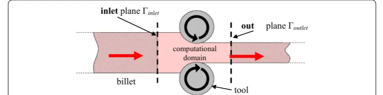
If only the steady-state is of interest, more specific formulations can be considered for reducing both computational times and memory. They have in common a great reduc-tion of the computareduc-tional domain, which is fixed in the flow direcreduc-tion [10], and an Eule-rian type of flow formulation (see Figure 1). It allows a better and more optimal control of the mesh size distribution without compromise on accuracy, in particular in the large gradients zones at the inlet and outlet of the roll bite. Domain geometry being unknown and closely coupled to material flow, its initial shape is often designed as the best possi-ble estimation of the final, steady-state, geometry of the product.
computational domain inletplane Γinlet
out plane Γoutlet
tool billet
Figure 1 Eulerian window around the forming zone for a rolling problem, definition of the inlet Ŵinput and
In the continuity of the Lagrangian approach, the steady regime can be incremen-tally computed using an Arbitrary Lagrangian or Eulerian (ALE) formulation inside the so-called Eulerian window, as in [11] so benefiting from the computational domain reduction and mesh adaptation [12]. However, the approach being basically the same (lagrangian step followed by mesh repositioning and field transfer), it still requires many time increments to properly propagate the domain deformation from the input plane to the output plane. Therefore the computational time is of the same order of magnitude (time reduction is only about 30% in [9] for the test case investigating in “Applications to metal forming problems” and 15% for a U channel with 6 stands [13]). Only the direct computation of the steady regime through directly solving steady-state problems equations allows reducing computing time by an order of magnitude or more [10, 14, 15].
In [16], Tortorelli and Balagangadhar introduced the reference frame concept that allows extending the ALE framework to steady-state problems. Within a displacement-based formulation, the domain geometry is directly computed by solving a multi-field problem and integrating state variables on the undeformed configuration. A simplified formulation was applied for welding [15], and also for drawing and rolling processes in 2D [17] using a penalty contact formulation instead of the more specific contact treat-ment initially developed in [16].
Within a velocity-based formulation, the multi-field steady-state problem was directly solved by Ellwood et al. [18] for simple polymer extrusion process. This fully coupled resolution is achieved by adding free surface conditions (29) to the mechanical problem and thus considering geometry corrections in addition to velocities and pressures. How-ever, due to strong couplings between material flow computation, free surface computa-tion and contact with tools constraining free surface correccomputa-tion a decoupled approach is preferred in literature [2, 5, 19]. It consists of a staggered fixed-point algorithm where the thermo-mechanical equations and convection equations are first solved for a given and fixed shape, and then the domain shape is corrected according to the newly com-puted material flow. Few iterations generally allow finding the domain shape, provided that the initial shape is not too distant from the final shape [4]. All these approaches only differ in the way the domain free surface is corrected, either by streamline integration, one by one, or by resolution of a global free surface problem.
The first approach is almost exclusively based on structured meshes, the nodes of which can be aligned along the streamlines, thus providing an easy and accurate way to integrate shape corrections [6]. Contact is a recurrent problem of these formulations. Contact equations are left aside during streamlines integration to avoid any discontinui-ties. A next step is therefore needed to project nodes on the tools using simple [20] or complex smoothing operations [5, 6].
The aim of the present work is to develop a steady-state formulation compatible with a velocity-based formulation, parallel computations and unstructured meshes. It is also expected to be sufficiently robust to handle all kinds of complex geometries met in metal forming applications. Therefore, the iterative fixed point approach is used to ensure compatibility with velocity formulation, and the free surface correction is computed through a global resolution to ensure compatibility with unstructured meshes and paral-lel computations.
“First step: position of the thermal-mechanical problem and velocity field compu-tation” presents the simple forming problem over a known domain; it consists of the thermo-mechanical equations of the metal forming problem. “Second step: free surface correction” gives a general description of the computation of the free surface correction for a known material velocity field with a non-null normal velocity, and presents differ-ent weak formulations used in literature. Section 4 introduces the new weak formulation for the free surface correction that shows necessary to handle complex contact condi-tions in 3D, along with the coupling of contact equacondi-tions between the two alternatively solved problems (simple forming problem and free surface correction). Resolution of simple analytical problems in “Evaluation on analytical tests” assesses the quality and robustness of several variants of the proposed formulation and “Applications to metal forming problems” applies the most promising one to actual metal forming problems.
First step: position of the thermal‑mechanical problem and velocity field computation
In this section, the shape of the computational domain is supposed to be known as its contact surface Ŵc, (the part of Ŵ=∂� that is both geometrically in contact with the forming tools and undergoing a negative contact pressure). The resolution of the thermo-mechanical equations aims at finding the steady-state velocity field associated to this domain and contact surface.
Conservation equation and boundary conditions Conservation equations: mechanics
The considered formulation is presently restricted to hot forming processes where the elastic part of the deformation can be neglected [23]. The material is assumed to be incompressible. Inertia can also be neglected because of low acceleration forces in com-parison to the plastic forces [2, 5]. The Cauchy stress tensor σ and the velocity v satisfy the equilibrium and volume conservation Eq. (1)
The constitutive equation is written for s, the deviatoric part of σ and follows the Nor-ton–Hoff model (2).
(1)
∇ ·σ =0 in ∇ ·ν=0 in
(2)
s=σ+pI=f(ε¯,ε˙¯,T)=2K(ε¯,T)
�√ 3ε˙¯
�(m−1) ˙
ε
p= −1 3tr(σ )
T is the temperature, ε˙ the strain rate tensor, ε˙¯ the equivalent strain rate, ε¯ the equiv-alent strain (3) and K(ε¯,T) the material consistency, which is here supposed to only depend on T and ε¯ to model temperature softening and strain hardening or softening.
During this resolution, the geometry (free surface) and boundaries (contact surface) of the domain are thus assumed to be known. The free surface condition is written on Ŵf through Eq. (4), where n is the outside normal to the surface. On the contact surface
Ŵc, non-penetration conditions are expressed, in a steady and Eulerian framework for a unilateral contact, by the Signorini conditions in (5), where νtool is the tool velocity, and friction is modeled by the velocity-dependant Norton law (6) where νs is the sliding velocity, αf and p the friction coefficients.
Domain upstream and downstream boundaries
Inlet and outlet planes (Figure 1) of the computational domain are introduced arbitrarily. The conditions written there are therefore more or less artificial. To avoid perturbations, it is therefore necessary to apply these conditions far enough from the plastic deforma-tion zone, at a posideforma-tion where it can be ascertained than the material flow is a Rigid Body Motion (RBM), i.e. the gradient of the velocity field is null there. Two implementations are proposed in [6]:
– stress-based the stress vector in these boundary planes is set to the average tension stress at each point (FE node), the shear component being zero:
– velocity-based the in-plane velocity is cancelled (8) and the normal velocity (in the main flow direction) is imposed homogeneous on the Sect. (9); there remains one equation to write to obtain a well-posed problem, the integral of the stress normal to the section is set equal to the imposed tension force (10).
(3) ˙
ε=1
/2(∇ν+t∇ν); ˙¯ε=2/3 √
˙
ε: ˙ε; ¯ε= t=tend
t=tbeg ˙¯ εdt.
(4)
σn=0 on Ŵf
(5)
(σn)·n ≤0
v−vtool·n ≤0 on Ŵc ⇒ ((σn)·n)
v−vtool·n=0 on Ŵc
(6)
τ= −αfK�∆vs�p−1∆vs on Γc
(7) σ·n=Ftension/S
(8) v−(v·n)n=0
(9) vi·n=vj·n ∀i,j∈Ŵinlet (Ŵoutlet)
(10)
Ŵinlet
σndS=Ftension
Here, the first (stress-based) formulation is used and furthermore Ftension = 0 for simplicity.
The weak forms of these equations [24] provide a mixed velocity and pressure formu-lation that is summarized by:
This set of equations is discretized using tetrahedral finite element with the quasi-lin-ear P1+/P1 “mini element” interpolation [25] satisfying the compatibility condition [26]. Contact is enforced by a penalty method using a node-to-facet formulation [24].
Conservation equation: energy
Within a steady-state formulation, time partial derivative vanishes so thermal equations only consist of convection and diffusion terms (12) associated to a source term w˙ result-ing from a fraction of the plastic strain power σ: ˙εpl dissipated during mechanical work:
where ρ is the density, c is the specific heat and k is the material conductivity.
On the inlet surface, the initial temperature is imposed (either homogeneous, or a map obtained by computing former history…).
On the free surface, there are thermal exchanges with the environment by convection and radiation. They are modeled by the Fourier law presented in Eq. (13a). On the con-tact surface, heat is produced by friction and exchanged by conduction (13b):
where hconv is the convection transfer coefficient, εr is the material emissivity, σr is the Stefan–Boltzmann constant, hcond is the conduction exchange coefficient with tools, bm and btool respectively are the material and tool effusivities (b=
k.ρ.c), while Text and Ttool respectively denote the ambient and tool temperatures that are supposed constant here.
In the temperature steady-state Eq. (12), convection is dominating conduction because of high Péclet numbers [3, 6]. In this case, a standard Galerkin formulation produces numerical oscillations. They are avoided by appealing to a Streamline Upwind Petrov– Galerkin (SUPG) formulation [27] that is more precisely presented in “Second step: free surface correction”. The resulting weak form of thermal equations is summarized by:
State variables equations
For state variables, similarly, time partial derivatives vanish so that time integration results into pure convection problems. With the considered constitutive model (2) only the equivalent strain rate (3) needs to be integrated into the equivalent strain (15) by tak-ing into account the initial values εimp¯ of ε¯ on Ŵinlet:
(11) R(x,Ŵc,ε¯,T,v,p)=0
(12)
ρcv· ∇T =k�T + ˙w in �
(13) q·n= −k∇T ·n=
hconv(T−Text)+εrσr
T4−Text4 on Ŵf
hcond(T−Ttool)− bm
bm+btool(
τ·�vs) on Ŵc
(14)
T(x,Ŵc,ε¯,v,T)=0
(15)
v· ∇ ¯ε= ˙¯ε in � ¯
¯
ε (and more generally any state variable, such as e.g. pertaining to microstructural, metallurgical models) and ε˙¯ are computed at integration points so their finite element discretization are not continuously interpolated. With the P1+/P1 quasi-linear interpola-tion used here, ε˙¯ can be regarded as piecewise per element or P0. In order to avoid using a more complex and not necessarily more accurate discontinuous Galerkin method as in [15], it is preferred to project the P0 equivalent strain rate ε˙¯ onto a P1 continuous linear mapping in order to use the standard SUPG formulation to solve Eq. (15) and then to use the P1 linear continuous interpolation of ε¯ to compute the equivalent strain values at integration points. Referring to [28], this method provides accurate results and allows using the same resolution method as for the temperature equation.
Finally, integration of state variable equations can be symbolically summarized as:
Thermo‑mechanical coupling
For the applications studied, thermo-mechanical coupling is not very strong so rather than directly solving the full (ε¯,T,v,p) problem, which increases very significantly the problem size, equations are solved in an iterative manner until convergence, as follows:
However, the algorithm is not suited for more complex thermo-mechanical iors such as Friction Stir Welding (FSW), continuous casting or elasto-plastic behav-iors. Some changes have to be made to help the convergence. Adding simple relaxation methods for reducing potentially large changes can be highly beneficial. For even more stronger coupling behavior, sub fixed points should be added to insure the thermo-mechanical convergence at each iteration [6].
Second step: free surface correction
In this section, the velocity field v is supposed to be known and to be the solution of the steady-state flow on the considered domain, which needs to be corrected in order to sat-isfy the free surface condition (18).
Governing equations
When the flow is steady, the velocity field is tangential to the surface Ŵ of the domain ; streamlines of surface particles are on the surface and there is no material flow through this surface. In other words, the normal component of the velocity field is null on Ŵ, which provides the fundamental equation for the stationarity of the free surface (18).
where n(x) is the outside normal of Ŵ at x, and v is the velocity field on . If this condi-tion is not satisfied with the current posicondi-tion X of the surface shape (v·n(X)�=0), then
X must be corrected by a displacement t (19) in order that Eq. (18) is satisfied.
(16)
L(x,v,ε)¯ =0
(17)
Given�x(i),Ŵc(i) �
:
−compute�v(i+1),p(i+1)�from: R�x(i),Ŵ(i)
c ,ε¯(i),T(i),v(i+1),p(i+1) �
=0
−computeT(i+1)from: T�x(i),Ŵc(i),ε¯(i),v(i+1),T(i+1) �
=0
−computeε¯(i+1)from: L�x(i),v(i+1),ε¯(i+1)�=0
(18)
Following the bibliography and previous works [2, 6], a fixed-point algorithm is used to solve the steady-state equations. Therefore, in this section, the dependence of v on t is neglected [19], just like x was supposed to be independent of v in the previous section, so that: ν=ν(X)=ν(x).
On the input surface, supposed “far enough” that the movement is a RBM and the sec-tion is perfectly known, Ŵinlet (see 1), the points are fixed (20), t = 0. On the output sur-face Ŵoutput, the points have to remain in the plane but must move in it for searching the unknown final section; their correction t is thus tangent to Ŵoutput (20).
In many works of literature [2, 22, 29] the free surface correction (FSC) problem is simplified by imposing that the correction t is collinear with the normal of the surface n(X) (21), leading to a one degree of freedom formulation.
After finite element discretization, the normal vector n(x) (22) is not defined at the finite element nodes but it can be computed on any surface facet by:
where (ξ,η) denotes the local coordinates system of the surface facet.
It can be noticed that u(t) is linear with respect to t, if t has a fixed and constant direc-tion, and that it is quadratic with respect to t in the general case.
Contact condition
The corrected surface also has to satisfy the non-penetration Eq. (23) on Ŵf, where h(t)
(24) is a linear approximation of δ(x), the signed distance of x to the closest tool (nega-tive if the point penetrates the obstacle and posi(nega-tive otherwise).
where ntool denotes the inside normal to the tool surface.
This unilateral contact condition is not sufficient because it does not prevent the com-plete release of all contact conditions during the free surface correction [20] leading to oscillations or even divergence. It proves necessary to enforce a bilateral contact condi-tion (25) on ŴcFSC, the contact surface of Ŵ. It is defined using both the sign of contact normal stress associated to the current velocity field and the penetrations occurred after the free surface correction (its definition is presented into more details in “Contact con-ditions transmission between velocity field computation and free surface correction”).
(19)
x=X+t on Ŵ
(20)
x=X on Ŵintlet t·noutlet=0 on Ŵoutlet
(21)
t=t·d with d≈n(X)
(22)
n(x)= u(x)
�u(x)� where: u(x)≡u(t)= ∂x ∂ξ ∧
∂x ∂η
(23) h(t)≥0 on Ŵf
(24)
Turning now to the tangential plane, if a sticking contact condition is applied on ŴcFSC [22], chances are that the mesh degenerates (as described in [29]). Hence, a sliding bilat-eral contact condition is preferred (25).
Weak formulation
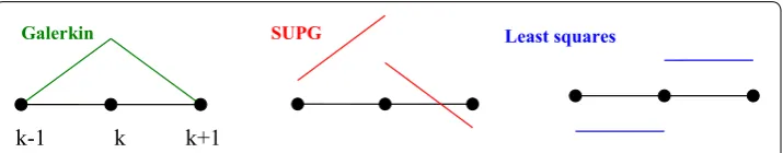
Different weak formulations of Eq. (18) are encountered in literature: the standard Galerkin formulation is used in [2], while the stabilized SUPG form is preferred in [22] and the least square approach is selected in [19]. In the case where t has a single degree of freedom per node as in (21), all these variants can be gathered under a generic form (26) with different choices for the test functions N*:
Galerkin and SUPG formulations are characterized by different choices for N∗, namely:
where le and ve respectively are characteristic element length and velocity. These values are simply the average of segments length and nodal velocity of a triangle.
The Galerkin formulation amounts to using N∗=NGalerkin=N (28), where N is the isoparametric finite element shape function. For problems more complex than those presented in [2], this formulation often leads to an indeterminate system of equations. In fact, the free surface Eq. (18) results in a pure convection problem of the surface correc-tion t from the input plane. The SUPG formulation is therefore much better adapted [22, 30] as the solution is stabilized by involving the flow direction in the test function NSUPG (28) [upwind facets have more weight in the formulation (see Figure 2)].
An alternative to SUPG, least square (LS) formulation [19] consists in minimizing the integral of the square of Eq. (18) which leads to a parabolic problem. In the present work, the formulation is slightly modified (29) in order that the resulting system of equations is linear in the simple cases when d (21) is constant.
(25)
h(t)=0 on ŴcFSC
(26) ∀N∗, r(t)=
Ŵfinal
N∗(ν·n(t))dSfinal=
Ŵref
N∗(ν·u(t))dξdη
(27)
with:dSfinal= � u(t)� �u0�
dSinitial and dSinitial= �u0�dξdη
(28)
NGalerkin=N NSUPG =N+ 1 2
le ve(
v· ∇N)
k k+1
k-1
Galerkin SUPG Least squares
The differentiation of (29) provides a system of equations similar to Eq. (26) where N∗=NLS (30)
It can be noticed that the LS formulation naturally extends to the case where t is a vec-tor with several degrees of freedom. Both SUPG and LS formulations provide non sym-metric weights (see Figure 2) which enable them to handle the convection terms.
Contact Eqs. (23) and (25) are imposed at the finite element nodes by a node-to-facet penalty formulation:
where tk is the surface correction of node k and Sk is the associated surface, Sk = Ŵ
NkdS. The operator [x]+= 1
2(|x| +x) keeps only positive values. ρcFSC is a specific penalty coef-ficient for the free surface correction (FSC) which is set to 10,000. This value was chosen empirically and leads to a great accuracy without any convergence difficulties.
Volume mesh regularization
The correction of node positions on the domain surface causes distortions of the volume mesh or at least degeneration of its quality. In order to maintain the elements quality during the free surface iterations, a volume mesh regularization is carried out by using a Laplacian operator. The volume mesh correction t is the solution of the linear Laplace Eq. (32) subjected to imposed values on the entire mesh surface, resulting from the free surface correction.
New formulation for free surface correction
As discussed in “Weak formulation”, the Galerkin formulation is limited to specific and rather simple configurations; both Galerkin and SUPG formulations are well adapted when the correction t is a scalar, while the LS formulation allows an easy extension to 3D problems when t is a vector. However, studies of analytical problems (see “Evaluation on analytical tests”) show that the LS formulation is not converging to the expected solution when contact is taken into account and when the flow is significantly oriented. There-fore, the LS formulation should be improved to be applied to 3D forming problems. Two modifications are presented hereafter.
(29) Min
t
(Φ(t)), Φ(t)= 12
Ŵ(
v·u(t))2dξdη
(30) NLS=
v·∂u
∂t
(31)
Min ���� t
(Φc(t)), withΦc(t)= 12ρcFSC
� k∈Ŵf
Sk[h(tk)]+2+ �
k∈ŴFSC c
Skh(tk)2
(32)
�t =0 in �
Upwind least square formulation
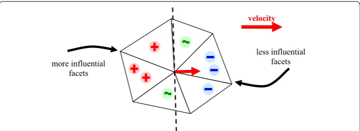
As mentioned in “Weak formulation”, the free surface correction can be regarded as a convec-tion problem, so that the flow direcconvec-tion has to be taken into account in the test funcconvec-tions of the weak equations as in the SUPG formulation. The least square formulation also provides a dissymmetry in the flow direction but gives the same absolute values to the weights of the up-flow and down-flow. Therefore, a new formulation aiming at combining the advantages of the LS and SUPG formulations is developed. It consists in modifying the LS equivalent test function N∗=NLS (30) by introducing in the definition of the normal (vector u) a sensitivity to its position with respect to the flow, as presented in Figure 3 and in Eq. (34), through the Ck coefficient (−1≤Ck ≤1) calculated like in the SUPG formulation (34).
The resulting formulation is called LS_supg because its shape functions (33) combine the SUPG shift with LS shape function:
The (1+Ck) coefficient is equal to 2 for perfectly upwind facets and to 0 for perfectly downwind facets. Thus, except these very particular facets, all other facets contribute to the weak form (see schematic representation of Figure 4), contrary to the streamline integration approach where only upwind terms contribute. Therefore, another variant to the LS formulation is considered by only taking into account the upwind terms (see Figure 4). Its shape functions (34) combine the streamline integration approach with LS shape function, so it is called LS_sl:
It should be noticed that the matrices symmetry of the LS formulation is consequently lost with these new formulations.
(33)
u∗(t)=u(t)+
k=1,3
Ck
∂u(t) ∂tk tk
, with Ck = ∇
Nk·vk �∇Nk� · �vk�
(34) NLS_ supg =(1+Ck)
v· ∂u
∂tk
(35)
NLS_sl =[Ck]+
v· ∂u ∂tk
velocity
less influential facets more influential
facets
Figure 3 Upwind shift in the calculation of the weights for the LS_SUPG formulation—flow is from left to
Full 2 degrees of freedom (DoF) formulation
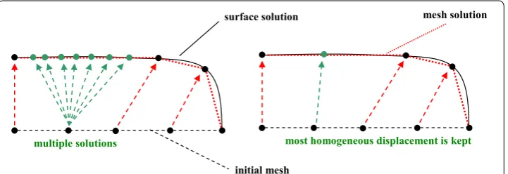
A free surface algorithm with only one degree of freedom per node reduces its field of appli-cation to only simple processes and geometries. It is mainly due to the displacement direc-tions that do not always coincide with the real displacements. Calculation of these direcdirec-tions is an intuitive guess based on the last geometry from the iterative algorithm. It is thus com-plicated to predict the displacement of an edge (Figure 5). Adding a second degree of free-dom makes the search of the directions automatic. Furthermore, it introduces the possibility of more complex displacements, which is useful for mesh regularization (Figure 5).
The least squares formulation can easily be extended to two degrees of freedom. Each Eq. (36) is computed from the differentiation of the normal velocity functional (29) in each direction. Whereas it is more complex for the SUPG formulation as only one equa-tion per node can be calculated. Thus, the SUPG formulaequa-tion is set aside. For the ease of the implementation, three degrees per node are set and a penalization method is used to cancel the displacements in the rolling direction (38a), or in the flow direction (38b) for a more general formulation. The penalty factor ρd is set to 100. This value is not set to high because slight displacements in the flow direction are not problematic.
However, this increase of the number of degrees of freedom leads to ill-conditioned problems. For instance, surface nodes can slide freely along the solution surface with-out making any change of the functional (29) (Figure 6). Therefore it is necessary to introduce a criterion for obtaining a solution. In this work, smoothed displacements are favored, which is done by adding a Laplacian operator for the diffusion of corrections t in each spatial direction ei (39). In order to preserve the free surface solution, a relative
(36)
∀t∗∈Ŵ, r(t)= ∂Φ(t) ∂t∗ =
Ŵ
v·∂u(t) ∂t∗
(v·u(t))dξdη.
LS_supg LS_sl
Figure 4 Schematic representation of LS_supg (left) and LS_sl (rigth) test functions at node k in pseudo‑1D when the flow is from left to right.
Initial section Solution section
Displacements for 1 degree of freedom Displacements for 2 degrees of freedom
tool
billet
cross section
symmetry planes
small weight wr is used in Eq. (37) which already contains free surface, contact and DoF reduction problems. This solution provides surface mesh regularization, which is very useful when domain corrections are large.
Unfortunately, the algorithm is extremely sensitive to the regularization weight wr. For small values, the problem is ill-conditioned and fails to converge. For larger values that make the convergence possible, the impact of regularization on the free surface solution is far from negligible. Therefore, the stabilization is only applied to the Newton–Raphson corrections, as presented in Eq. (40). In this way, the non-linear equations of the problem are not changed by the regularization, which only affects the corrections within the New-ton–Raphson iterations, so the algorithm converges toward a solution of the free surface equations without any compromise. On the other hand, this approach increases the num-ber of Newton–Raphson iterations, but as most of the computational cost is spent for the resolution of the velocity calculation, this additional cost is not significant.
Contact conditions transmission between velocity field computation and free surface correction
During the first step, velocity computation (VC) (“First step: position of the thermal-mechanical problem and velocity field computation”), the contact surface Ŵc is assumed to be known, while during the free surface correction (FSC) (“Second step: free surface
(37)
Φ′(t)=Φ(t)+Φc(t)+Φd(t)+wrΦr(t)
(38) Φd(t)= 12ρd
k∈Ŵ
dimp·t2; Φd(t)= 1
2ρd
k∈Ŵ v
k·t �vk�
2
(39)
∂Φr(t)
∂t ≡�t=0⇒
∀k∈Ŵ
∀i= {1, 2, 3} ,rk,i(t)=
Ŵ
∇Nk· ∇(t·ei)dS=0.
(40)
H(i)+wrH(i)r t(i+1)−t(i)
= −r(i)with r= ∂
Φ′−wrΦr
∂t and H =
∂r ∂t initial mesh
multiple solutions most homogeneous displacement is kept surface solution mesh solution
correction”), bilateral contact conditions are enforced on ŴFSCc . The coupling between these two contact surfaces is a master key for the convergence of the fixed-point algo-rithm. However, each step is not self-sufficient to detect accurately the contact area. The chosen algorithm gradually establishes the contact during iterations by both the velocity calculation and the free surface correction. Using a penalty method for non-penetration conditions leads to the calculation of two nodal contact forces, one for each stages: VC
k and FSC
k . It is worth mentioning that penalty weights are not similar, the VC is a rough problem and its coefficient has to be lowered to 100.
At the first iteration, Ŵcinit is defined geometrically from the initial domain shape, by the contact distance (41). This contact zone is then used for the resolution of the velocity field calculation to apply unilateral contact (5) and friction (6) conditions. From the pen-alty formulation, with ρc the contact penalization factor, the resolution allows computing contact forces VC
k at any node k (42). During the free surface correction, these contact forces define the zone ŴcFSC(42) where a sliding bilateral contact condition is applied (25). It should be noted from Eq. (23) that the non-penetration equations are always enforced for free surface nodes. Symmetrically to the velocity field calculation, a pseudo-contact force FSC
k can be defined at any node k (43) after the free surface correction. The contact surface ŴcVC is now defined by (43) for the next iterations.
For a forming problem like the rolling application of Figure 7, the contact zone is the intersection between ŴVCc and ŴcFSC (44). The contact forces from the velocity calculation
VC
k allow releasing the contact nodes downstream of the obstacle (but not upstream because they happen to be always negative). On its part, the pseudo-contact forces FSC
k from the free surface correction allow releasing the contact nodes upstream the obstacle [but they are not reliable as a criterion to release downstream nodes because of the coef-ficient ε in (43)].
(41)
Ŵinitc =
k∈Ŵ, δ(Xk) <0
(42)
ŴFSCc =
k∈Ŵ, VC
k <0
, withVC
k = −ρcVC vk−vktool
·ntool k
+
(43) ŴVCc =
k∈Ŵ, FSC
k <0
, with FSC
k = −ρcFSC[ε−h(t)]+
(44)
Ŵc=ŴFSCc ∩ŴVCc
velocity calculation
free surface calculation
It is worth mentioning for the calculation of FSC
k in Eq. (43) that the free surface cor-rection equations are not mechanical equations, so that it is more questionable to con-sider FSC
k as a real contact force; it is rather related to the accuracy of the free surface movement. Consequently, it shows necessary to introduce a numerical pseudo-adhesion coefficient ε in the definition of FSC
k . In practice, ε is taken equal to 2% of the mesh size.
Evaluation on analytical tests
Presentation of the tests
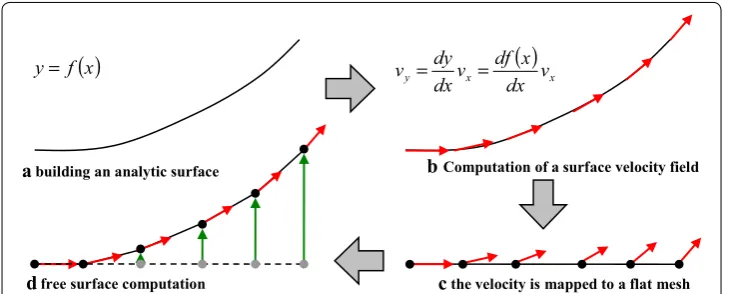
The free surface correction is calculated for several analytical test cases involving different dif-ficulties in order to assess the accuracy of the weak formulations, the contact treatment and the application to 3D problems with edges. All the analytical problems are built according to the same scheme, presented in Figure 8. First, a long 2D sheet is deformed in the vertical direction by an analytical function f (y = f(x)) (Figure 8a). The tangent vector is analytically computed at each node of the deformed sheet (Figure 8b) and is used to define the velocities of the nodes of the undeformed sheet (Figure 8c), the free surface correction problem is now posed (Figure 8d). Its resolution should provide the original shape of the deformed sheet.
DoF test cases
A smooth surface is obtained using a Gaussian function for f(x) (Eq. (45a) and Figure 9 top). For a more complex pattern a bidimensional sine-shaped function with growing amplitude is developed ((45b) and Figure 9 bottom).
In order to first compare the different weak formulations, only one degree of freedom per node is authorized, in the direction normal to the flattened mesh. Thus the Laplacian regularization (39) can be omitted. 2D meshes of respectively 6000 and 36,000 nodes are used to evaluate the finite element convergence of the methods tested.
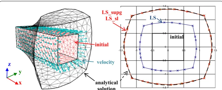
DoF test case with edges
A three-dimensional test case is set: a square section is progressively enlarged (Figure 10 right) by following a quadratic function in the direction normal to the surface (46). For this problem, the Laplacian smoothing procedure (39) is enabled. To prevent displacements in (45)
(a)y=5 exp(−0.01(x−40)2) (b)y=0.05xsin(πx)sin(πz)
( )
x fy= y x
( )
vxdx x df v dx dy v = =
d free surface computation c the velocity is mapped to a flat mesh b Computation of a surface velocity field a building an analytic surface
the x direction, the functional (38a) is used. The Galerkin and SUPG are not tested because this problem has two degrees of freedom per node.
DoF test cases with contact
For the Gaussian function (45a), a tool is set to bound the upward movement (Figure 11). This obstacle can be considered as a flat sheet parallel to the flattened mesh placed at a height about 2.5 mm, i.e. half the expected displacement. During the resolution, pen-etrations occur and enable the unilateral contact condition. The resulting solution has to respect both free surface and contact conditions.
Results for test cases without contact
For test cases with only one DoF, a simple criterion is used to quantify solutions accuracy (47), while it is more complicated for the test case with edges as the mesh regularization makes nodes slide on the surface. Instead of comparing directly correction displacements, (46) r=r0+0.1x2
5 mm 10 mm
100 mm
10 mm fixed nodes
main velocit direction
x
y z
Figure 9 Analytical surfaces: Gaussian function (top), sine function (bottom).
analytical solution x
y z
-1.5 -1 -0.5 0 0.5 1 1.5
-1.5 -1 -0.5 0 0.5 1 1.5
LS LS_supg
LS_sl
initial
velocity initial
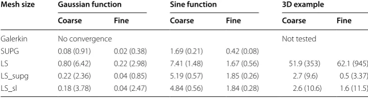
the closest distance of the solution for outlet nodes is used. Table 1 summarizes the results for both test cases with one and two DoF for both infinite and L2 norms.
DoF test cases
On these test cases, the Galerkin method (28a) fails to converge (see Table 1). LS_supg and LS_sl (resp. (33) and (34)) are either as accurate (sine function) or more accurate (Gaussian function) as the LS formulation. The SUPG formulation (28b) is the most accurate because it has the best nodal accuracy on the sheet edges, whereas least squares methods tend to smooth the solution. In other words, these nodal boundary conditions are more favorable to Galerkin-like formulations.
DoF test case with edges: effect of mesh smoothing
The convergence of the LS formulation is significantly affected by the Laplacian smooth-ing for 3D examples (Table 1). Nonlinear corrections decrease significantly at each iteration, making the convergence really slow. Even after 60 nonlinear iterations, the solution is far from the exact solution (Figure 10 right) and the convergence appears to be blocked. The introduction of an upwind shift solves this non-convergence issue. Ls_ supg and Ls_sl formulations give accurate results within less than 20 iterations (Table 1): the surface is precisely retrieved, the edges are perfectly preserved and the mesh is prop-erly regularized (Figure 10).
(47)
Θk =
tk−tkth tmaxth
Solution with no tool
Least squares formulation
Upwind formulations Obstacle
rolling direction
v.n 0
Figure 11 Adding a horizontal tool shows up physical and non‑physical behavior if an upwind formulation is used or not.
Table 1 Error (%) for nodes position displacement on analytical test cases for different refinement of 2D meshes
Infinite and L2 (in parenthesis) norms are presented.
Mesh size Gaussian function Sine function 3D example Coarse Fine Coarse Fine Coarse Fine
Galerkin No convergence Not tested
SUPG 0.08 (0.91) 0.02 (0.38) 1.69 (0.21) 0.42 (0.08)
Interaction with contact
The LS formulation is unable to compute the expected shape (see Figure 11).
Although this formulation is sensitive to the flow direction, it is not sensitive to its orientation so the contact information is transported both downwind and upwind. The contact equations are satisfied but the contact area is underestimated; the nor-mal component of the velocity is minimized all over the domain but the formula-tion does not succeed to cancel it; an unexpected shape is consequently obtained (see Figure 11). On the other hand, contact and free surface conditions are per-fectly satisfied all over the domain for all the upwind formulations, not only the SUPG formulation but also for the newly LS_supg and LS_ls formulations. It is worth mentioning SUPG and LS_supg tend to create really slight oscillations on the free surface before the contact area. These oscillations are proportional to the discontinuities introduced by contact constraints, which can be regarded as Dir-ichlet conditions. For non-fully upwind formulations some strategies exist to pre-vent these problems [31]. However, these oscillations can be neglected in forming processes applications where the material flow and the contact conditions are not fully incompatible; they do not introduce any discontinuities.
Summary
To sum-up, Galerkin formulation does not converge on the test cases chosen (the problem solution is not unique) while SUPG formulation provides the most accurate results on such analytical functions. LS-based formulations are properly converging toward the exact solution with decreasing finite element mesh size, and their accuracy is quite satisfactory. These formulations can be easily extended to 3D problems with a correction vector (rather than a scalar in a prescribed direction) where they make it possible to properly preserve the problem shape edges without requiring specific techniques to detect and deal with these surface singularities, a difficult and hazardous issue. When contact comes into play, the original LS formulation has a non-physical behavior resulting from the lack of a direction for contact corrections propagation. Introducing an upwind shift, either with the LS_supg or LS_sl formulation allows fix-ing this issue while preservfix-ing or even improvfix-ing the accuracy of the LS formulation. Therefore, the following forming applications will be studied using LS_sl. Even if LS_ supg seems better, a full upwind formulation is preferred for avoiding issues with con-tact like the original LS formulation.
Applications to metal forming problems
Introduction
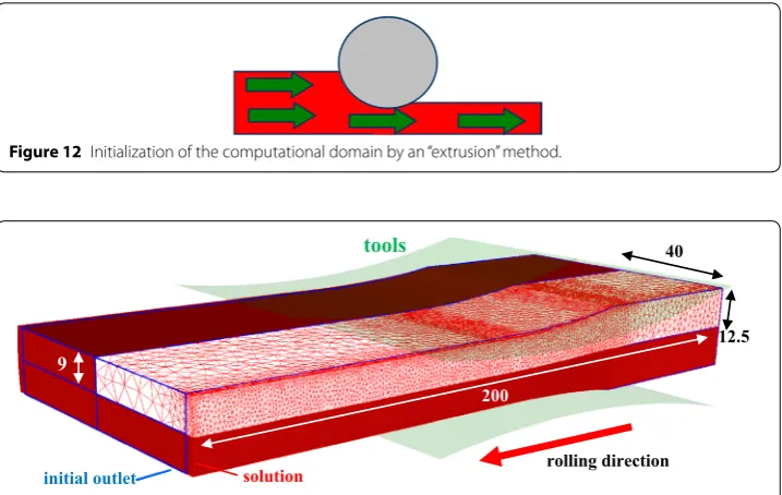
The Eq. (38b) is used to penalize any corrections along the material flow. The initial com-putation domain is constructed with an “extrusion” method (Figure 12), giving an almost optimal initialization. The construction can be obtained by extruding the input plane in the forming direction through the tool set, in order to create a sequence of sections that are then connected together. When nodes of a section penetrate an obstacle, their posi-tion is projected back on its surface. The “extrusion” approach is used in the following applications, as presented in Figures 13 and 14 schematized in Figure 12.
Rolling of thick plate
A thick metal sheet is rolled as presented in Figure 13. The tools are cylinders with a 600 mm diameter and separated by 18 mm. Their rotational velocity is about 27.5 rpm. This problem includes an edge, the displacement of which should not be restricted to the mesh surface normal direction. Consequently, a 1 DoF approach would fail and a more general free surface formulation is required. Two symmetry planes are used to reduce the problem size (Figure 13). A coarse mesh of about 5000 nodes and a finer one with 15,000 nodes (Figure 13) are used for the computations.
The geometries of the final section obtained with non-steady Forge®, steady Lam3 on the finer mesh and both meshes for the LS_sl formulation are very similar (Figure 15). By looking more closely at the zoom of Figure 16, it first appears that reference solutions proposed by Lam3 and Forge® differ. It can be explained by the use of different finite ele-ments (tetrahedron versus hexahedral) where the hexahedra happen to be stiffer (they do not formally satisfy the velocity/pressure compatibility condition). Moreover, it could be caused from the non-similar implementation of behavior and friction laws, or even from the integration methods: streamlines versus time step. However the difference is only about 0.2 mm for a 3 mm widening. Comparing solutions with the same finite (48)
K=30; m=0.15; αf =0.3; p=0.15
Figure 12 Initialization of the computational domain by an “extrusion” method.
tools
200
40
12.5
rolling direction
9
initial outlet solution
elements, results are very close. Solution obtained with the finer mesh provides a very good conservation of the edge profile, which is also in excellent agreement with the non-steady solution of Forge® (Figure 16).
initial outlet
solution
Figure 14 Simulation of a rolling process “oval to square” with a steady state formulation. The computational domain is only ¼ of the billet.
Figure 15 Initial and final sections obtained for the simulation of thick plate rolling process.
Rolling of long product
A case of rolling process “oval to square” is studied and presented in Figure 14. The input section is an oval with main axis 108 mm and small axis 36 mm. Reduction brings the maximum height axis to 56 mm. These tools have a 600 mm diameter, are separated by 3.5 mm and have a rotational velocity of 48 rpm. Similarly to the previous simulation, two symmetry planes are used (Figure 14). This problem is a tough challenge for evaluating the conservation properties of free surface algo-rithms because the domain is very long (1,000 mm), the section reduction rate and shape change are very high and the contact area is much harder to compute than in previous problem due to more complex tools. With this problem, the Lam3 soft-ware gets stuck in its convergence. The algorithm periodically sets a portion of a “stream line” in contact and then releases it. Lam3 solution does not vary at the end because of high relaxations enabled for handling major contacts changes. With the present formulation, a first coarse mesh (of about 5,000 nodes) finds difficulty to correctly propagate the bar enlargement from the tools exit to the output plane: the upper free surface is slightly flattened (see Figure 17). A much more refined mesh (of about 40,000 nodes—Figure 14) provides very accurate solution which is in excellent agreement with non-steady Forge® (Figure 17).
Convergences and speeds‑up
In all the tests, and particularly in the two rolling problems presented, the free surface algo-rithm converges toward the solution within a reasonable number of iterations, about 50, as presented in Figure 18 for the bar rolling. However, it can be noticed that an approximate and rather coarse solution can be quickly found after less than 15 iterations but that 25 or more additional iterations are needed to reach an accurate and stable solution (Figure 18).
Figure 17 Left initial and final shapes obtained for the simulation of shape rolling “oval to square”. Right
In fact, mesh regularization is conflicting with the resolution of the free surface equations, so close to the problem solution, the regularization induces slight mesh displacements along the free surface, of about 1% of the mesh size, which results into additional iterations. For too much iteration, it can lead to a degenerated mesh since no criterion is used to enforce the mesh quality. Anyway, the obtained accuracy is fully consistent with the finite element size and precision of the penalty contact formulation.
The volume loss on the final configuration for each formulation is presented in Table 2. For the incremental formulation, it is simply a comparison between initial and final mesh volume (49), whereas for iterative formulations, inlet and outlet material fluxes are considered as in Eq. (50). A finer mesh leads to a better accuracy and a reduction of the volume loss for the thick plate test case. However, for the shape rolling test case it does not produce the expected improvement. Indeed, in this particular configuration, the coarse mesh simplifies the surface curvatures helping the free surface algorithm to convect the section shape. Using a finer mesh means the curvatures are still present and have to be transported. However, the mesh is not fine enough to deal with unstructured topology. As the convection is more complex for the free surface algorithm, the mesh regularization appears to smooth the shape progressively in the rolling direction. Solv-ing this problem is the scope of a new formulation which would be detailed in a future paper.
(49)
Vincremental=
Vfinal−Vinit
Vinit
Figure 18 Convergence of the shape rolling “oval to square”.
Table 2 Volume loss (%)
Thick plate Shape rolling
Incremental 0.115 0.40
Lam3 0.008 0.38
Steady‑state (coarse) 0.260 0.45
Directly computing the steady state using an iterative approach however brings impor-tant speed-ups with respect to the incremental computation of this regime. In fact, in transient computations time steps must be small enough to be consistent with the expected accuracy in the contact area, whereas in steady state modelling, the domain inlet and outlet must be set sufficiently far away from the plastic deformation zone. Both result in an increase of the total number of times step, in addition to the increase of the size of the computational domain. For the thick plate simulation, the steady-state version of Forge® is 8 times faster than the incremental version (see Table 3). It can be noticed that it requires more iterations and more nodes than the Lam3 software, so making it less efficient. On the other hand, the software is stopped when the maximum number of 100 iterations is reached but the solution is not fully satisfactory. In this case, the speed-up with respect to the incremental approach is even more impressive (see Table 4) because the domain length is much larger: the steady-state version is 21 times faster than the transient computation with Forge®.
Sensitivity to domain initialization
In steady-state formulations, initialization of the computational domain may become tricky because of its influence on the convergence. Less iterations are needed if the initial geometry is closer to the solution, but also convergence may not be reached if the initial geometry is too far or not adequate as in the “oval to square” example with Lam3 or as mentioned by Mori [10]. It is important to figure out that the formulation developed in this article is based on a small correction approach. From an engineering standpoint, it is crucial to have a robust method that is able to converge from almost any reasonable initial solution satisfying the basic boundary conditions.
An almost optimal initialization of the computational domain can be obtained by the “extrusion” method (Figure 12), which was used in previous cases. For the purpose of testing the approach robustness, two non-optimal methods are analyzed.
Both start from a simple extrusion of the input plane without taking care of the tools. A first approach consists in lifting the tools up so that they are no longer in contact with (50)
�Viterative=
Qinlet+Qoutlet
Qinlet
with Qinlet=
Ŵinlet�
v· �ndS Qoutlet =
Ŵoutlet�
v· �ndS
Table 3 CPU times for the simulation of thick plate rolling
Number of nodes Number of iterations/increments CPU time Speed up
Incremental 10,000 → 16,000 280 2 h 57 min 1
Lam3 12,000 28 5 min 35
Steady‑state 15,000 40 22 min 8
Table 4 CPU times for the simulation of “oval to square” rolling
Number of nodes Number of iterations/increments CPU time Speed up
Incremental 20,000 → 37,000 1099 24 h 45 min 1
Lam3 12,000 100 38 min 39
the workpiece, then moving them back to their original position by performing a non-steady forging simulation (Figure 19a). Another simple approach consists in deleting all the finite elements that penetrate inside the obstacle before projecting new surface nodes on the tool surface (Figure 19b). Boundary conditions are thus properly enforced by these last two methods although the height of the downstream part of the workpiece is far from being correct. Moreover, the spread between the tools is significantly overes-timated by the forging method, as shown in Figures 20 and 21.
The first application case is studied again, raising the sliding friction coefficient αf from 0.3 to 0.5 with the three different possible initializations (see the outline of the initial shape produced by forging in Figure 20). Figure 22 shows that the free surface algorithm is robust enough to converge for all of them, toward very similar solutions that are pre-sented in Figure 20. Obviously, the convergence is faster with the extruded initial geome-try. The other two methods are quite comparable. The observed convergence oscillations are only 1% of mesh size in magnitude. It is noticed that the different sections obtained (Figure 20) are quite comparable up to the finite element accuracy.
Similarly, the three different initializations are used to study the robustness of the algorithm for the second and more complex application problem. Figure 21 left shows that here again, the algorithm converges towards almost the same solution whatever the initial geometry, even if it is very far from the final solution, as shown in Figure 21 top–right with the forged initial shape. This robustness property mainly results from the mesh regularization introduced inside the free surface algorithm; it acts like a relaxa-tion and allows a progressive convergence toward the final shape, as shown in Figure 21 bottom–right.
forging material removing
Figure 19 Different ways for initializing the computational domain: forging, material removing.
0 2 4 6 8 10
41.8 42 42.2 42.4 42.6 42.8 43 43.2 43.4 width (mm)
height (mm)
Lam3
steady-state extrusion steady-state forging steady-state removing
Conclusion
An iterative approach for the search of continuous processes steady state has been pre-sented in this paper. The aim was to reduce computational times encountered with incre-mental formulations by searching directly the steady state with a staggered algorithm. A staggered fixed-point algorithm is used where a first velocity field is solved for on a fixed and known geometry, and then a domain correction is performed. The second stage is controlled by a free surface calculation that needs to be solved in the most general way in terms of mesh type (unstructured), geometries complexity and parallel computation compatibility. A global resolution using the finite elements method and two DoF satisfies all imposed constraints.
Simple analytical test cases with only one DoF evidence the purely convective aspect of the free surface problem. Thus, shape functions for the variational problem have
initial
iteration 49 0
5 10 15 20 25 30
0 5 10 15 20 25
width (mm)
height (mm)
incremental steady-state extrusion steady-state forging steady-state removing
Figure 21 Left, final shapes calculated from different initializations with a steady state formulation. Right, visualization of both initial and final geometries for a “forging” initialization.
1.00E-03 1.00E-02 1.00E-01 1.00E+00 1.00E+01
0 5 10 15 20 25 30 35 40
Max correction on the outlet (mm)
iterations
steady-state extrusion (coarse)
steady-state extrusion (fine)
steady-state forging (fine)
steady-state removing (fine)
to take into account the flow direction. Two new weak formulations based on the LS method, for facilitating the transition to a 2 DoF algorithm, and using SUPG advantages are developed in this study: LS_supg and LS_sl (streamline-like). However, LS_sl takes benefit from its fully upwind formulation to eliminate the oscillations which could occur with imposed contact constrains.
Using a two DoF formulation in the cross section helps to generalize the free surface algorithm by handling mesh singularities, like edges where displacement directions can-not be easily guessed. To obtain a solution, a Laplacian operator is added to the free surface problem introducing a mesh regularization. The final algorithm retrieves the geometry with accuracy while preserving edges and mesh quality.
Contact equations are considered during the free surface calculation by using both unilateral and sliding bilateral conditions. The second condition prevents a complete loss of contact and is possible through the mesh regularization. A contact analysis is then crucial to enforce the coupling between the two stages of the staggered fixed-point algo-rithm. Detection of compressed nodes is performed progressively by using specific and complementary data from both mechanical and geometrical resolution stages.
The developed algorithms were applied with success on various analytical test cases and for material forming processes like shape rolling. Accuracies are similar to the unsteady formulation and important speeds-up are gained, ranging from 10 to 20. The method appears to be robust even when using on purpose non-optimal initial domains to increase the convergence difficulty.
However, the two DoF formulation for the free surface computation has too much freedom leading to some issues: relatively slow convergence of the free surface calcu-lation, parasite displacements after both geometry and contact are stabilized. Adding more control upon each DoF by making a differentiation between surface and edge nodes during the free surface calculation would correct these problems, as the first ones need one DoF to be optimal whereas the last ones require a second DoF. This is subject of a future paper.
Authors’ contributions
LF designed the study. With JLC, they supervised and guided the work, and offered appreciated insight on the industrial software Forge3. UR developed the iterative algorithm, ran the different test cases and conducted the detailed analysis. LF and UR drafted the manuscript, and JLC helped its reviewing. All authors read and approved the final manuscript.
Author details
1 Transvalor, 694 avenue Maurice Donat Parc de Haute Technologie, 06250 Mougins, France. 2 MINES ParisTech, PSL
Research University, CEMEF, CNRS UMR 7635, CS 10207 rue Claude Daunesse, 06904 Sophia Antipolis Cedex, France. Acknowledgements
Support for this work has been provided by the “Forge‑ALE” project gathering several companies of the metal forming industry (Ascometal‑CREAS, AREVA‑CEZUS, Aubert&Duval, Industeel and Ugitech). Their financial and technical support is gratefully acknowledged. Helps from Transvalor, in particular C. Béraudo and E. Perchat, during the development of a steady version of Forge® were much appreciated. We also want to thank Pierre Montmitonnet for helpful comments while writing the paper.
Compliance with ethical guidelines Competing interests
The authors declare that there are no conflicts of interest.
References
1. Mori K, Osakada K (1984) Simulation of three‑dimensional deformation in rolling by the finite‑element method. Int J Mech Sci 26(9–10):515–525
2. Lee Y‑S, Dawson PR, Dewhurst TB (1990) Bulge predictions in steady state bar rolling processes. Int J Numer Meth‑ ods Eng 30(8):1403–1413
3. Vacance M, Massoni E, Chenot JL (1990) Multi stand pipe mill finite element model. J Mater Process Technol 24:421–430
4. Sola G, Vacance M, Massoni E, Chenot J‑L (1994) Thermomechanical simulation of seamless tube rolling using a 3D finite element method. J Mater Process Technol 45(1–4):187–192
5. Kim HJ, Kim TH, Hwang SM (2000) A new free surface scheme for analysis of plastic deformation in shape rolling. J Mater Process Technol 104(1–2):81–93
6. Hacquin A, Montmitonnet P, Guillerault J‑P (1996) A steady state thermo‑elastoviscoplastic finite element model of rolling with coupled thermo‑elastic roll deformation. J Mater Process Technol 60(1–4):109–116
7. Hacquin A, Montmitonnet P, Guillerault JP (1998) A three‑dimensional semi‑analytical model of rolling stand defor‑ mation with finite element validation. Eur J Mech A Solids 17(1):79–106
8. Abdelkhalek S, Zahrouni H, Potier‑Ferry M, Legrand N, Montmitonnet P, Buessler P (2009) Coupled and uncoupled approaches for thin cold rolled strip buckling prediction. Int J Mater Form 2(S1):833–836
9. Fourment L, Gavoille S, Ripert U, Kpodzo K (2013) Efficient formulations for quasi‑steady processes simulations: Multi‑mesh method, arbitrary Lagrangian or Eulerian formulation and free surface algorithms. In: Zhang SH et al (eds) Proceedings of NUMIFORM 2013, Shenyang, China, Aip Conference Proceedings, vol 1532, pp 291–297 10. Mori K, Osakada K (1990) Finite element simulation of three‑dimensional deformation in shape rolling. Int J Numer
Methods Eng 30(8):1431–1440
11. Wisselink HH, Huétink J (2004) 3D FEM simulation of stationary metal forming processes with applications to slitting and rolling. J Mater Process Technol 148(3):328–341
12. Donea J, Huerta A, Ponthot J‑P, Rodríguez‑Ferran A (2004) Arbitrary Lagrangian–Eulerian methods. In: Stein E, de Borst R, Hughes TJR (eds) Encyclopedia of computational mechanics, vol 1. Wiley, ISBN 0‑470‑84699‑2 13. Boman R, Ponthot J‑P, Barlat F, Moon YH, Lee MG (2010) New Advances in numerical simulation of stationary
processes using arbitrary Lagrangian Eulerian formalism. Application to roll forming process, vol 1252, no. 1. AIP Publishing, pp 133–140
14. Kim SY, Lee HW, Min JH, Im YT (2005) Steady state finite element simulation of bar rolling processes based on rigid‑ viscoplastic approach. Int J Numer Methods Eng 63(11):1583–1603
15. Geijselaers H (2003) Numerical simulation of stresses due to solid state transformations: the simulation of laser hardening. PhD Dissertation, University of Twente
16. Balagangadhar D, Dorai GA, Tortorelli DA (1999) A displacement‑based reference frame formulation for steady‑state thermo‑elasto‑plastic material processes. Int J Solids Struct 36(16):2397–2416
17. Yu Y (2005) A displacement based FE formulation for steady state problems. PhD Dissertation, University of Twente 18. Ellwood KRJ, Papanastasiou TC, Wilkes JO (1992) Three‑dimensional streamlined finite elements: design of extrusion
dies. Int J Numer Methods Fluids 14(1):13–24
19. Chenot JL, Montmitonnet P, Bern A, Bertrand‑Corsini C (1991) A method for determining free surfaces in steady state finite element computations. Comput Methods Appl Mech Eng 92(2):245–260
20. Yamada K, Ogawa S, Hamauzu S, Kikuma T (1989) 3D analysis of mandrel rolling using RP‑FEM. In: Thompson EG et al (eds) Proceedings of NUMIFORM 89, Fort Collins, USA. A.A. Balkema, Rotterdam
21. Vacance M (1993) Modélisation tridimensionnelle par éléments finis du laminage à chaud des tubes sans soudures. PhD Dissertation (in French), ENSMP
22. Ramanan N, Engelman MS (1996) An algorithm for simulation of steady free surface flows. Int J Numer Methods Fluids 22(2):103–120
23. Montmitonnet P (2006) Hot and cold strip rolling processes. Comput Methods Appl Mech Eng 195(48–49):6604–6625
24. Chenot J‑L, Fourment L, Coupez T, Ducloux R, Wey E (1998) Forge3 (R)—a general tool for practical optimization of forging sequence of complex three‑dimensional parts in industry. In: International Conference on Forging and Related Technology (ICFT 98). Professional Engineering Publishing, pp 113–122: ISBN: 1–86058–144–7
25. Coupez T, Marie S (1997) From a direct solver to a parallel iterative solver in 3‑d forming simulation. Int J High Per‑ form Comput Appl 11(4):277–285
26. Brezzi F, Fortin M (eds) (1991) Mixed and hybrid finite element methods, vol 15. Springer, New York
27. Brooks AN, Hughes TJR (1982) Streamline upwind/Petrov–Galerkin formulations for convection dominated flows with particular emphasis on the incompressible Navier–Stokes equations. Comput Methods Appl Mech Eng 32(1–3):199–259
28. Basset O, Digonnet H, Guillard H, Coupez T (2005) Multi‑phase flow calculation with interface tracking coupled solu‑ tion. In: Papadrakakis M et al (ed) Proceedings of COUPLED PROBLEMS 2005, Santorin, Greece, CIMNE, Barcelona 29. Chenot JL, Montmitonnet P, Buessler P, Fau F (1991) Finite element computation of spread in hot flat and shape roll‑
ing with a steady state approach. Eng Comput 8(3):245–255
30. Soulaïmani A, Fortin M, Dhatt G, Ouellet Y (1991) Finite element simulation of two‑ and three‑dimensional free surface flows. Comput Methods Appl Mech Eng 86(3):265–296