Structured and Sparse Annotations for Image Emotion Distribution Learning

(1)

The Thirty-Third AAAI Conference on Artificial Intelligence (AAAI-19)

Structured and Sparse Annotations for Image Emotion Distribution Learning

Haitao Xiong,

1

_{Hongfu Liu,}

2

_{Bineng Zhong,}

3

_{Yun Fu}

4

1_{School of Computer and Information Engineering, Beijing Technology and Business University, Beijing, China} 2_{Michtom School of Computer Science, Brandeis University, Waltham, USA}

3_{chool of Computer Science and Technology, Huaqiao University, Xiamen, China} 4_{Department of Electrical and Computer Engineering, Northeastern University, Boston, USA} [email protected], [email protected], [email protected], [email protected]

Abstract

Label distribution learning methods effectively address the la-bel ambiguity problem and have achieved great success in im-age emotion analysis. However, these methods ignore struc-tured and sparse information naturally contained in the anno-tations of emotions. For example, emotions can be grouped and ordered due to their polarities and degrees. Meanwhile, emotions have the character of intensity and are reflected in different levels of sparse annotations. Motivated by these ob-servations, we present a convolutional neural network based framework called Structured and Sparse annotations for im-age emotion Distribution Learning (SSDL) to tackle two chal-lenges. In order to utilize structured annotations, the Earth Mover’s Distance is employed to calculate the minimal cost required to transform one distribution to another for ordered emotions and emotion groups. Combined with Kullback-Leibler divergence, we design the loss to penalize the mis-predictions according to the dissimilarities of same emotions and different emotions simultaneously. Moreover, in order to handle sparse annotations, sparse regularization based on emotional intensity is adopted. Through combined loss and sparse regularization, SSDL could effectively leverage struc-tured and sparse annotations for predicting emotion distribu-tion. Experiment results demonstrate that our proposed SSDL significantly outperforms the state-of-the-art methods.

Introduction

For the reason that an image can contain rich semantics, many people tend to use images to express their opinions and emotions. So, it is important to find out the emotions im-plied in images, especially for social network sites like Twit-ter and so on (Zhao et al. 2016; Yang, She, and Sun 2017; Zhao et al. 2018b). In traditional image emotion analysis, an image is in general associated with one or more emotion labels, which belong to single-label and multi-label learn-ing methods (Zhang and Zhou 2014). However, there exists an ambiguity problem for this task, which means the uncer-tainty of the ground-truth label (Yang, Sun, and Sun 2017; Zhao et al. 2018a). Moreover, images often express mix-ture of different emotions and different people may have totally different emotional feelings. Through single-label and multi-label learning, the relative importance of differ-ent emotions in description of the image is not clear. For this

reason, label distribution learning methods are designed to reveal the extent to which each label describes the samples through label distribution prediction and have achieved great success (Geng 2016; Yang, Sun, and Sun 2017; Zhao et al. 2018a). Label distribution learning can provide an alternate view of learning process, where each sample is mapped to a label distribution instead of a single label or multiple labels. Recently, convolutional neural networks (CNNs) based la-bel distribution learning methods have shown superior per-formance of distribution prediction against traditional label distribution learning methods (Yang, She, and Sun 2017).

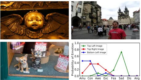
Unfortunately, most of label distribution learning based image emotion analysis methods rarely utilize characters of emotions. On the one hand, emotions have the character of polarity and are presented in varying degrees (Mikels et al. 2005). This means that emotions can be grouped and or-dered. Ordered emotions and emotion groups are presented in structured annotations. Here we take seven emotions in Emotion6 dataset (Peng et al. 2015) for example. These emotions have ordered sequence according to the degrees of positive or negative polarity. Besides, these emotions can be divided into three groups with different polarities, which are positive group, neutral group and negative group. In image emotion analysis, mis-prediction of one emotion as nearby emotion, such asjoyandsurprise, is more adorable than as far away emotion, such as joy and sadness. Fig-ure 1 shows polarity and group information in seven emo-tions from Emotion6 dataset. Red-based and gray-based col-ors are used to represent different degrees of positive and negative polarity, while white color is used to represent neu-tral polarity. On the other hand, emotions also have the char-acter of intensity (Sheppes et al. 2014) and are reflected in different levels of sparse annotations. Figure 2 shows three images from Flickr LDL dataset (Yang, Sun, and Sun 2017) and the emotion distribution line chart of these images. Flickr LDL has eight emotions which areamusement, con-tentment,awe,excitement,fear,sadness,disgustandanger. The first four belong to thepositive groupand the last four belong to thenegative group. In the line chart, emotions are in ordered sequence from emotion amusement to emotion

(2)

posi-Joy Surpr

ise

N

eut

ral

Fe

ar

S

adne

ss

D

isgus

t

A

nge

r

Polarity

Positive Negative

Positive Group Neutral Group Negative Group

Figure 1: Polarity and group information in seven emotions from Emotion6 dataset.

tive groupresulting in non-zero group sparse annotations of emotion groups. Emotional intensity of the bottom left im-age is weaker than the top right imim-age, because there exist one emotion in thepositive groupis not shown in the bot-tom left image resulting in spare annotations of emotions in thepositive group. As shown in Figure 1 and Figure 2, there exist polarity and intensity characters among the emo-tions, which refers to structured and sparse information in annotations of emotions. However, most label distribution learning methods use Kullback-Leibler (KL) divergence as loss to measure the similarity between the ground-truth and the predicted label distribution (Yang, She, and Sun 2017; Geng 2016). Consequently, these methods can hardly cap-ture the polarity and intensity characters of images emotion, which makes it difficult to learn precise emotional represen-tations for explaining the image emotions. Therefore, how to effectively use image emotional characters in label distri-bution learning still remains a big challenge.

In this paper, we develop a deep model to handle the above challenges. For utilization of structured annotations in emotional polarity, the Earth Mover’s Distance (EMD) is employed to calculate the minimal cost required to trans-form one distribution to another for ordered emotions and emotion groups. Then we design the combined loss based on EDM and KL divergence to penalize the mis-predictions according to the dissimilarities of same emotions and dif-ferent emotions simultaneously. Moreover, we design the sparse regularization based on emotional intensity to han-dle different levels of sparse annotations. Through combined loss and sparse regularization, structured and sparse annota-tions could be effectively leveraged for learning. Our contri-butions are summarized as follows. First, we design a novel CNN-based framework called Structured and Sparse anno-tations for image emotion Distribution Learning (SSDL) to analyze image emotions, which integrates information of structured and sparse annotations into a CNN based model for effectively learning. Second, structured annotations are effectively utilized via combining the EMD and KL diver-gence in loss. Furthermore, sparse regularization based on emotional intensity is designed to handle the sparse annota-tions of emoannota-tions. Experimental results demonstrate the su-perior results of SSDL compared with several state-of-the-art methods in image emotion distribution learning.

Related Work

Image Emotion Classification

Through the development of computer vision, image emo-tion classificaemo-tion has been an interesting and meaningful

Figure 2: Three images from the Flickr LDL dataset are an-notated in eight ordered emotions. The line chart on bottom right shows emotion distributions of these images.

research topic recently. The solutions mainly concentrate on two kinds of approaches: dimensional models and categor-ical models. Dimensional models use a few basic spaces for emotion description, and the categorical models classify emotion into one of the typical emotion categories, which are obvious for common people understanding and thus have been mainly used by most previous work. According to that whether the image can be associated with one or more emo-tion labels, categorical models can be divided into single-label and multi-single-label classification (Cambria et al. 2017; Zhang and Zhou 2014). Feature extraction is an important factor that affects the analysis performance and low-level features of image are most used (Zhao et al. 2014b). These features can be generated automatically, but lack in describ-ing emotions. So hand-crafted features based on art and psy-chology theory are proposed and show better performance than low-level features in several situation, such as emotions in art images (Zhao et al. 2014a). Due to the different bene-fits of these features, fused multi-modal features are gener-ated for image emotion analysis (Zhao et al. 2017).

On the other side, deep models like CNNs have shown strong ability to generate high-level features automatically (Chen, Zhang, and Allebach 2015; Zhao et al. 2018c). Mean-while, these features show good performance in many com-puter vision tasks (Wang et al. 2016). So, CNN-based meth-ods have been frequently employed in emotion classifica-tion and show great success. In order to use large scale yet noisy training data to, solve the emotion prediction, Youet al.designed a robust CNN-based model called Pro-gressive CNN (PCNN) for visual sentiment analysis and got obvious improvement (You et al. 2015). Architecture-Frame-Transformer Emotion Classification Network (FT-EC-net) was proposed in (Tripathi et al. 2017) to solve three highly correlated emotion analysis tasks: emotion recogni-tion, emotion attribution and emotion-oriented summariza-tion. However, these work did not consider structured anno-tations of ordered emotions.

Label Distribution Learning

(3)

the samples through label distribution prediction, and has been a hot topic in machine learning. Generally speaking, current label distribution learning methods can be roughly generalized into three strategies which are problem trans-formation, algorithm adaptation and designing specialized algorithms (Geng 2016). Representative methods build on problem transformation strategy include, SVM and PT-Bayes, which come from traditional classification methods SVM and Naive Bayes (Geng 2016). Through algorithm adaptation strategy, classification algorithms, such as kNN and backpropagation (BP) neural network, can be naturally extended to deal with label distributions (Geng 2016). Geng

et al. adopted designing specialized algorithms strategy to propose SA-IIS, SA-BFGS and SA-CPNN for label distri-bution learning (Geng, Yin, and Zhou 2013; Geng 2016).

Recently, with the development of CNNs, CNN-based methods are proposed for label distribution learning. Deep label distribution learning (DLDL) method utilized the la-bel ambiguity in both feature learning and classifier learning (Gao et al. 2017). Experiments showed that even when the training set is small, DLDL could still achieve better per-formance for age estimation. Specially for image emotion analysis, convolutional neural network regressions (CNNR) based on CNN with Euclidean loss for each emotion was presented in work of Ref. (Peng et al. 2015). Through nor-malization, the regression results were transformed to prob-abilities of all emotions. Yanget al.proposed a deep CNN approach through joint optimization of image emotion clas-sification and distribution learning , and the model showed better performance (Yang, She, and Sun 2017).

Problem Definition

Given an input image, we are interested in predicting emo-tion distribuemo-tion considering structured and sparse annota-tions of image emoannota-tions. Assume that we have C emo-tions e = {e1, e2, ..., eC}, and N images for training x = {x1, x2, ..., xN}. According to different emotional polarities, e can be divided into R emotion groups g =

{g1, g2, ..., gR}. For consideration of structured annotations of ordered emotions and emotion groups, the comparison operator between different emotions and emotion groups should be defined firstly. Suppose ei and ej are different emotions, we defineei≺ejwhich means the positive polar-ity degree ofeiis less thanej, and also means the negative polarity degree ofei is more thanej. Then we can define gm ≺gn which means the positive polarity degree of each emotion ingmis less than each emotion ingn. Through com-parison operator, image emotions can be reordered. If there is no special explanation,eare ordered emotions andg are ordered emotion groups. On the other hand, in order to ex-press sparse annotations of different levels of emotional in-tensity, we defineisas single strong emotional intensity,ig as group strong emotional intensity andiwas weakly strong emotional group intensity. Sois,igandiware collections of images fromxnandis∩ig∩iw=∅.

The probability distributiondxn={d

e1

xn, d

e2

xn, ..., d

eC

xn}of

emotions for the imagexnis regarded as the emotion distri-bution, wheredec

xnis the probability of emotionecfor image xnand represents the extent to which emotionecdescribes

xn.dexcnis under the constraintsd

ec

xn>0and

∑C

c=1d

ec

xn= 1

which mean that the emotion probability is non-negative and

e can describe the emotions of the image fully. Emotion group distributiondg

xncan be got by adding probabilities of

all emotions that belong to the same emotion group. Let us denote byf(xn;w)the activation values of the last fully connected layer for imagexn. And wis the weight. Specially,fec(xn;w)is the activation value for emotionec.

In order to reveal structured annotations representing by emotion groups, fgr(xn;w)is defined as the sum of

acti-vation values for all emotions in group gr. The network is trained by minimizing the following objective function:

w∗= argmin w

1

N N

∑

n=1

L(dxn, f(xn;w)) +R(w), (1)

whereL(·,·)is the suitable loss function for image emotion distribution learning, andR(·)is the proper regularization.

In image emotion distribution learning, the purpose of our proposed method is using structured sparse annotations to capture polarity and intensity characters for predicting emo-tion distribuemo-tion. In order to consider characters of image emotions in learning, we propose a deep CNN-based frame-work that can extract and integrate structured and sparse an-notations from polarity and intensity characters for learning. For challenge of reflecting image emotional characters in modeling of label distribution learning properly, structured and sparse annotations are used in the loss function and reg-ularization for image emotion distribution learning.

Image Emotion Distribution Learning

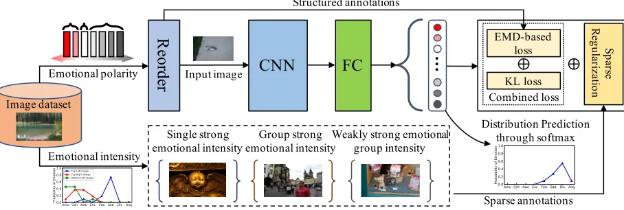
As illustrated in Figure 3, we design a deep CNN-based framework called Structured and Sparse annotations for im-age emotion Distribution Learning (SSDL), to utilize polar-ity and intenspolar-ity characters of emotions for learning. In the SSDL framework, image emotions are reordered according to the emotional character of polarity, then images are fed into a pre-trained CNN model with some modifications. The number of outputs of last fully-connected layer, which is classification layer, is assigned to the number of emotions. Through information of emotional polarity, SSDL extracts structured annotations from ordered emotions and emotion groups, which are used for EMD-based loss computing. Then EMD-based loss is combined with KL loss for pe-nalizing the mis-predictions according to the dissimilarities of same emotions and different emotions simultaneously. In addition, through information of emotional intensity based on ground-truth distributions, SSDL uses sparse annotations of different levels of emotional intensity for sparse regular-ization. Finally, combined loss and sparse regularization are both used for distribution learning optimization.

Combined Loss for Structured Annotations

(4)

CNN

FC

…

Image dataset

Sparse annotations KL loss EMD-based

loss Sp

ar

se

Re

gu

la

riz

ati

on

R

eor

de

r

Input image

Single strong emotional intensity

Group strong emotional intensity

Weakly strong emotional group intensity Structured annotations

Emotional polarity

Emotional intensity

Combined loss

Distribution Prediction through softmax

Figure 3: The deep framework of our proposed SSDL. SSDL extracts structured annotations from emotional polarity for EMD-based loss computing. Then EMD-EMD-based loss is combined with KL loss for penalizing the mis-predictions according to the dissimilarities of same emotions and different emotions simultaneously. Meanwhile, SSDL also uses sparse annotations of different levels of emotional intensity for sparse regularization.

which could lead to misclassification. Simply suppose there exist three ordered emotionse={e1, e2, e3}. The

ground-truth distributiond={0.6,0.2,0.2}, and two predicted dis-tributions aredˆ1={0.5,0.2,0.3}anddˆ2={0.5,0.3,0.2}.

The KL loss values between d, dˆ1 and d, dˆ2 are same.

However, in the case of image emotion analysis, the mis-prediction ofe1 as e2 ande3 should be different, and the

mis-prediction ase2 is more adorable because of the more

similarity betweene1ande2. To handle the above challenge,

EMD is employed which is defined as the minimum cost to transport the mass of one distribution to the other (Levina and Bickel 2001) and has shown better performance than softmax cross-entropy loss in ordinal classification prob-lems.

Firstly, for the reason of considering structured annota-tions of ordered emoannota-tions, EMD can be used to penalize mis-predictions of distribution according to distances of different emotions. As shown in problem definition, image emotions are ordered ase1 ≺e2 ≺... ≺eC, and we define the dis-tance between different emotionseiandejas|i−j|. Given the ground-truth distributiondand predicted distributiondˆ, the expression of EMD for emotions is defined as:

EMDe(d,dˆ) = ( 1

C C

∑

k=1

⏐

⏐CDFd(k)−CDF_dˆ(k) ⏐ ⏐

q

)1q_, ₍₂₎

where CDFd(k) means the cumulative distribution func-tion ∑k

c=1d

ec_{. Secondly, we also want to penalize}

mis-predictions of distribution between different groups. Or-dered emotions e can be divided into R ordered emotion groupsg as g1 ≺ g2 ≺ ... ≺ gR. The distance between different emotion groupsgiandgj is defined as|i−j|. The expression of EMD for emotion groups is defined as:

EMDg(dg,dˆg) = ( 1 R

R ∑

k=1

⏐

⏐CGDFdg(k)−CGDF_dˆg(k) ⏐ ⏐ q

)1q_, ₍₃₎

whereCGDFdg(k)means the cumulative group distribution

function∑k

r=1

∑

ec∈grd

ec_{. Finally, we use the EMD loss}

of emotions and emotion groups to generate the EMD-based loss for image emotion distribution learning:

LEM D= 1

CEMDe(d,

ˆ

d) + 1

REMDg(dg,

ˆ

dg), (4)

whereCis the number of emotions andRis the number of emotion groups.

For penalizing the mis-predictions according to the dis-similarities of same emotions and different emotions simul-taneously, loss functionL in SSDL combines EMD-based loss and KL loss through a weighted combination:

L=µLEM D+ (1−µ)LKL, (5)

whereLKL is KL loss and weightµ is used to adjust the importance of the two components in combined loss.

Regularization based on Emotional Intensity

Traditionalℓ1andℓ2regularizations are mainly used for

pre-venting over-fitting of training data. And ℓ1 regularization

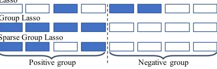
called Lasso (Cand`es and Wakin 2008) has the ability of pro-ducing sparse outputs at single-level. In order to get sparse outputs at group-level, group Lasso are proposed and show better performance in weight sparse learning (Baldassarre et al. 2016). Since group Lasso loses the guarantee of spar-sity at single-level, it may still be sub-optimal. To address this problem, sparse group Lasso considers sparsity at both single-level and group-level (Scardapane et al. 2017). As we known, images show different levels of emotional intensity reflected in sparse annotations. In order to reveal different levels of emotional intensity, we present sparse regulariza-tion using Lasso, group Lasso and sparse group Lasso.

(5)

Sparse Group Lasso Group Lasso

Positive group Negative group

Lasso

Figure 4: Comparison between Lasso, group Lasso, and sparse group Lasso for prediction. Blue square means the predicted probability of the emotion is non-zero.

and non-zeroed (blue squares) out by the corresponding pe-nalization. In Lasso example, three emotions are predicted in sparsity by removing emotions with optimizing single-level emotion considerations. Through group lasso, whole emo-tions inpositive group are predicted and none of emotions innegative groupare predicted. Sparse group Lasso exam-ple combines the usages of Lasso and group Lasso, and gets sparsity at single-level and group-level simultaneously.

The basic idea of sparse regularization based on emo-tional intensity is considering different emotion sparsities for sparse annotations of different levels of emotional in-tensity. Unlikeℓ1at single-level, emotion sparsity at

group-level forces all probabilities of emotions from the same group to be either all non-zeros, or all zeros. Specifically, we consider three different levels of emotional intensity:

• Single strong emotional intensity (is): as the emotions of top left image in Figure 2, there exists only single prominent emotion that an image shows, which can be understood as that the probability of this emotion exceeds the threshold and few emotions can describe the image;

• Group strong emotional intensity (ig): group strong emotional intensity means that emotions of the image are focused on all emotions from one emotion group, like the intensity of top right image in Figure 2.

• Weakly strong emotional group intensity (iw): not like the strict requirement of group strong emotional inten-sity, weakly strong emotional group intensity shows par-tial emotions from one emotion group, as the bottom right image in Figure 2 shows.

Forsingle strong emotional intensity, LassoRℓ1penalizes

the absolute magnitude of the predicted probabilities of all emotions, and is calculated as:

Rℓ1=∥f(xn, w)∥1=

C

∑

c=1

|fec(xn, w)|. (6)

Forgroup strong emotional intensity, group Lasso aiming at keeping the group sparse structure is suitable (Hu et al. 2017). The group sparsity of the predicted probabilities of all emotions with group structuregcan be measured through

ℓ2,1norm. Group LassoRℓ2,1is calculated as:

Rℓ2,1 = R

∑

r=1

∥fgr(xn, w)∥2=

R

∑

r=1

√ ∑

ec∈gr

(fec(xn, w)) 2_.

(7)

Forweakly strong emotional group intensity, only using Lasso or group Lasso cannot handle this emotional intensity. Sparse group Lasso keeps the group sparsity structure. At the same time, it permits single sparsity. Sparse group Lasso

Rsglis calculated by addingRℓ1 toRℓ2,1.

Sparse regularization Rsr uses Lasso, group Lasso and sparse group Lasso simultaneously for different levels of emotional intensity. The equation ofRsris given below:

Rsr=

∑

xn∈is

Rℓ1+

∑

xn∈ig

Rℓ2,1+

∑

xn∈iw

Rsgl. (8)

Moreover,ℓ2regularization∥w∥2is used to prevent

over-fitting. The overall regularizationRin SSDL is given below:

R=ξ1Rsr+ξ2Rℓ2(w), (9)

whereξ1andξ2are the regularization parameters to balance

the importance of the two components in objective function.

Experiments and Results

Implementation Details

To make this comparison, three image emotion distribu-tion datasets are selected, including Emodistribu-tion6 (Levi and Hassner 2015), Flickr LDL and Twitter LDL (Yang, Sun, and Sun 2017). Emotion6 is widely used as a benchmark dataset for emotion classification, which contains 1,980 im-ages collected from Flickr. Flickr LDL and Twitter LDL are two datasets collected mainly for emotion distribution learn-ing. Flickr LDL contains 11,150 images and Twitter LDL contains 10,045 images. In Emotion6, used emotions can be divided into three groups:positive,negativeandneutral group. In Flickr LDL and Twitter LDL, used emotions can be divided into two groups:positiveandnegative group. All datasets are randomly split into 75%training, 20%testing and 5%validation sets. The validation set is used for choos-ing the best parameters of our methods. The votes from the annotators are integrated to generate the ground-truth of im-age emotion distributiondthrough dividing votes for each emotions by total votes. If the probability of a single emo-tion exceeds0.6, these images have single strong emotional intensity. For the rest images, if the emotions shown in the image come from the same emotion group and all emotions in the group are shown, this image have group strong emo-tional intensity; if the emotions shown in the image come from the same emotion group but not all emotions in the group are shown, this images have weakly strong emotional group intensity.

In the experiments, SSDL is built on VGG-19 architecture (Simonyan and Zisserman 2014). We change the number of last fully-connected layer outputs to the number of emotions. The original loss layer is replaced by the combined loss. The learning rates of the convolution layers, the first two fully-connected layers and the classification layer are initialized as 0.001, 0.001 and 0.01. We fine-tune all layers by back propagation through the whole net using mini-batches of 32 and the total number of epochs is 20 for learning.

(6)

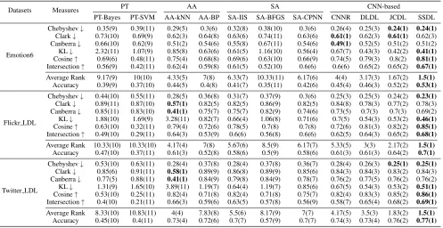
Table 1: Performance comparison between SSDL and the state-of-the-art methods for emotion distribution learning on Emo-tion6, Flickr LDL, Twitter LDL datasets measured by Chebyshev, Clark, Canberra, KL divergence, Cosine, Intersection, aver-age rank of all measures and accuracy.

Datasets Measures PT AA SA CNN-based

PT-Bayes PT-SVM AA-kNN AA-BP SA-IIS SA-BFGS SA-CPNN CNNR DLDL JCDL SSDL

Emotion6

Chebyshev↓ 0.35(9) 0.39(11) 0.29(5) 0.3(6) 0.32(8) 0.38(10) 0.3(6) 0.26(4) 0.25(3) 0.24(1) 0.24(1) Clark↓ 0.73(10) 0.69(9) 0.62(3) 0.64(8) 0.63(6) 0.74(11) 0.63(6) 0.61(1) 0.62(3) 0.61(1) 0.62(3) Canberra↓ 0.66(10) 0.62(9) 0.51(2) 0.54(6) 0.55(8) 0.67(11) 0.54(6) 0.49(1) 0.52(5) 0.51(2) 0.51(2) KL↓ 2.32(11) 1.07(9) 0.85(8) 0.63(6) 0.61(5) 1.16(10) 0.56(4) 0.67(7) 0.43(3) 0.42(2) 0.41(1) Cosine↑ 0.69(6) 0.48(11) 0.75(4) 0.68(8) 0.69(6) 0.63(10) 0.66(9) 0.74(5) 0.79(3) 0.8(2) 0.81(1) Intersection↑ 0.56(9) 0.42(11) 0.62(4) 0.59(8) 0.61(5) 0.52(10) 0.6(6) 0.6(6) 0.65(2) 0.65(2) 0.67(1)

Average Rank 9.17(9) 10(10) 4.33(5) 7(8) 6.33(7) 10.33(11) 6.17(6) 4(4) 3.17(3) 1.67(2) 1.5(1) Accuracy 0.39(9) 0.37(10) 0.44(5) 0.4(8) 0.41(7) 0.35(11) 0.42(6) 0.45(4) 0.46(3) 0.52(2) 0.53(1)

Flickr LDL

Average Rank 10.33(10) 10.33(10) 4.17(4) 7(8) 5.67(6) 8.5(9) 6.17(7) 5.33(5) 3(3) 2.17(2) 1.5(1) Accuracy 0.47(10) 0.37(11) 0.61(3) 0.52(8) 0.58(6) 0.5(9) 0.58(6) 0.61(3) 0.61(3) 0.64(2) 0.7(1)

Twitter LDL

Average Rank 8.33(10) 10.83(11) 4(4) 7.83(8) 5.5(6) 8.17(9) 7(7) 4.17(5) 3.5(3) 1.83(2) 1.5(1) Accuracy 0.45(10) 0.4(11) 0.73(4) 0.72(6) 0.7(7) 0.57(9) 0.7(7) 0.74(3) 0.73(4) 0.76(2) 0.77(1)

• Methods through problem transformation (PT): PT-Bayes and PT-SVM are based on traditional classification meth-ods SVM and Naive Bayes, and change the training sam-ples into weighted single-label samsam-ples for distribution learning (Geng 2016);

• Methods through algorithm adaptation (AA): traditional classification methods kNN and BP neural network are extended to deal with distribution learning and called AA-kNN and AA-BP (Geng 2016).

• Specialized algorithm methods (SA): SA-IIS uses a strat-egy similar to improved iterative scaling (IIS) that assum-ing the probability of each emotion to be the maximum entropy model (Geng, Yin, and Zhou 2013); SA-BFGS is based on IIS using the idea of an effective quasi-Newton method Broyden-Fletcher-Goldfarb-Shanno for improv-ing (Geng 2016); SA-CPNN is conditional probability neural network(Geng, Yin, and Zhou 2013).

• CNN-based methods (CNN-based): CNNR uses Eu-clidean loss for learning (Peng et al. 2015); DLDL uses KL divergence as loss function (Gao et al. 2017); a multi-task CNN-based framework through Joint image emotion Classification and Distribution Learning (JCDL) (Yang, She, and Sun 2017).

For PT, AA and SA methods, features extracted from the last fully connection layer based on VGGNet deep model (Simonyan and Zisserman 2014) are used for distribution learning. Moreover, PCA approach is also used to get the first 280 principal features for more comparable and ef-fective learning. All our experiments are carried out on a

NVIDIA GTX Titan Xp GPU with 12GB memory.

In order to compare different label distribution learning methods, measures should be able to calculate the aver-age distance or similarity between the ground-truth and pre-dicted label distributions. As suggested in (Geng 2016), six distribution learning measures are applied in our experi-ments including Chebyshev distance(↓), Clark distance(↓), Canberra metric(↓), and KL divergence(↓). The similar-ity measures include Cosine coefficient(↑) and Intersection similarity(↑). Down arrow ↓means lower is better, and up arrow ↑means higher is better. Moreover, since KL diver-gence is not well defined when zero occurs, we use a small valueϵ= 10−10to replace zero value. In addition, the maxi-mum values of Clark distance and Canberra metric are deter-mined by the number of emotions. For standardized compar-ison, we divided Clark distance by the square root of num-ber of emotions and divided Cannum-berra metric by the numnum-ber of emotions. Moreover, We can utilize the max emotion in ground-truth and predicted distributions as the single emo-tion label for classificaemo-tion. In this way, accuracy can be cal-culated by classification result of the max emotion.

Results and Analysis

(7)

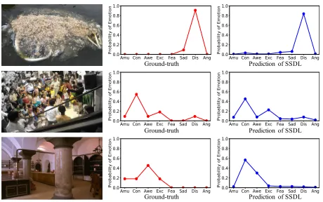
Ground-truth Prediction of SSDL

Figure 5: Predicted emotion distributions of SSDL on image examples are shown in last column. The ground-truth distri-butions is shown in the middle column.

Figure 6: Effect ofµfor combined loss on Emotion6 dataset. Note that µ = 1 means only using EMD-based loss, and

µ= 0means only using KL loss.

bold indicate the best values of each measure.

From the results, we can observe that: (1) SSDL shows su-periority in most of measures on all datasets and ranks first on all average rank measures, which demonstrates the ef-fectiveness of SSDL in image emotion distribution learning by leveraging structured and sparse annotations; (2) SSDL achieves the best max emotion classification performance, even though the main goal of our proposed method SSDL is predicting the emotion distribution. (3) for Clark and Can-berra measures, SSDL shows worse performance than AA-kNN because that AA-AA-kNN predicts emotion distribution depending on k nearest samples and is suitable for predicting emotions with low probabilities which are beneficial to the improvement of Clark and Canberra; (4) four CNN-based methods rank top 5 performance except that the performance of CNNR in few measures, which reveals the strong capacity of CNNs in image emotion distribution learning.

Several images from Flickr LDL dataset are shown in Figure 5, followed by the ground-truth and predicted emo-tion distribuemo-tion by SSDL. From the results, we can see that SSDL predicts distribution similar to the ground-truth dis-tribution and captures the sparse annotations of emotions. Specially, predicted distribution of the bottom image in Fig-ure 5 demonstrates that mis-predictions of SSDL for the im-age mainly move to nearby emotions in thepositive group

which is caused by the usage of EMD-based loss.

On Sensitivity of Combined Loss Parameter µ. In

Table 2: Effect of sparse regularization Rsr for SSDL on Emotion6 dataset.

Methods KL divergence↓ Cosine↑

SSDL(withoutRsr) 0.43 0.79

SSDL(withRsr) 0.41 0.81

SSDL,µcontrols the relative importance between the EMD-based loss and KL loss. The bigger value of µ, the more important of EMD-based loss. We use Emotion6 and three measures, which are KL divergence, Cosine coefficient and Accuracy, to demonstrate howµinfluences the performance of SSDL on Emotion6. The results are presented in Figure 6. From the curves, we find that: (1) the performance of only using EMD-based loss or KL loss is worse than using both as a combined loss, which illustrates that EMD or KL diver-gence can only handle the one aspect of the dissimilarities and using both can improve performance of distribution pre-diction; (2) performance of combined loss is effective and stable when increases µfrom 0.5 to 0.8, which means ad-dressing the usage of EMB-based loss. Through these re-sults, we can find out that our proposed combined loss is robust for image emotion distribution learning in SSDL.

On Effect of Sparse Regularization Rsr. In order to check the effect of sparse regularization in SSDL, we per-form experiments on Emotion6 using SSDL with and with-out sparse regularizationRsr. KL divergence and Cosine co-efficient are used for performance comparing. Firstly, we set

ξ1 = 0 to get SSDL without Rsr. Secondly, we use both components of regularization to get SSDL withRsr. Then we compare these methods and the results are shown in Ta-ble 2. From the results, we can detect that the performance of SSDL in emotion distribution learning is improved by us-ing sparse regularization, which reveals the effectiveness of

Rsrby capturing different levels of sparse annotations.

Conclusion

In this paper, we explored how to effectively use structured and sparse annotations in image emotion distribution learn-ing. A novel CNN-based framework named Structured and Sparse annotations for image emotion Distribution Learning was proposed, in which emotional characters of polarity and intensity are effectively considered. Combined EMD-based and KL loss were used to take structured annotations into account for emotional polarity. Meanwhile, sparse regular-ization was designed to take sparse annotations into account for emotional intensity. Extensive experiments on distribu-tion datasets revealed that the effectiveness of SSDL in im-age emotion distribution learning through utilizing rich in-formation extracted from structured and sparse annotations.

Acknowledgements

(8)

References

Baldassarre, L.; Bhan, N.; Cevher, V.; Kyrillidis, A.; and Sat-pathi, S. 2016. Group-sparse model selection: Hardness and relaxations. IEEE Transactions on Information Theory

62(11):6508–6534.

Cambria, E.; Poria, S.; Gelbukh, A.; and Thelwall, M. 2017. Sentiment analysis is a big suitcase. IEEE Intelligent Sys-tems32(6):74–80.

Cand`es, E. J., and Wakin, M. B. 2008. An introduction to compressive sampling. IEEE Signal Processing Magazine

25(2):21–30.

Chen, M.; Zhang, L.; and Allebach, J. P. 2015. Learning deep features for image emotion classification. In Image Processing (ICIP), 2015 IEEE International Conference on, 4491–4495. IEEE.

Gao, B. B.; Xing, C.; Xie, C. W.; Wu, J.; and Geng, X. 2017. Deep label distribution learning with label ambiguity.IEEE Transactions on Image Processing26(6):2825–2838. Geng, X.; Yin, C.; and Zhou, Z. H. 2013. Facial age estima-tion by learning from label distribuestima-tions.IEEE Transactions on Pattern Analysis and Machine Intelligence35(10):2401– 2412.

Geng, X. 2016. Label distribution learning. IEEE Trans-actions on Knowledge and Data Engineering 28(7):1734– 1748.

Hu, Y.; Li, C.; Meng, K.; Qin, J.; and Yang, X. 2017. Group sparse optimization via lp, q regularization. Journal of Ma-chine Learning Research18:1–52.

Levi, G., and Hassner, T. 2015. Emotion recognition in the wild via convolutional neural networks and mapped binary patterns. InProceedings of the 2015 ACM on International Conference on Multimodal Interaction, 503–510. ACM. Levina, E., and Bickel, P. 2001. The earth mover’s dis-tance is the mallows disdis-tance: Some insights from statis-tics. InComputer Vision, 2001. ICCV 2001. Proceedings. Eighth IEEE International Conference on, volume 2, 251– 256. IEEE.

Mikels, J. A.; Fredrickson, B. L.; Larkin, G. R.; Lindberg, C. M.; Maglio, S. J.; and Reuter-Lorenz, P. A. 2005. Emo-tional category data on images from the internaEmo-tional affec-tive picture system. Behavior research methods37(4):626– 630.

Peng, K. C.; Chen, T.; Sadovnik, A.; and Gallagher, A. C. 2015. A mixed bag of emotions: Model, predict, and transfer emotion distributions. InCVPR, 860–868.

Scardapane, S.; Comminiello, D.; Hussain, A.; and Uncini, A. 2017. Group sparse regularization for deep neural net-works.Neurocomputing241:81–89.

Sheppes, G.; Scheibe, S.; Suri, G.; Radu, P.; Blechert, J.; and Gross, J. J. 2014. Emotion regulation choice: a conceptual framework and supporting evidence.Journal of Experimen-tal Psychology: General143(1):163.

Simonyan, K., and Zisserman, A. 2014. Very deep convolu-tional networks for large-scale image recognition.Computer Science.

Tripathi, S.; Acharya, S.; Sharma, R. D.; Mittal, S.; and Bhattacharya, S. 2017. Using deep and convolutional neu-ral networks for accurate emotion classification on DEAP dataset. In AAAI Conference on Artificial Intelligence, 4746–4752.

Wang, J.; Yang, Y.; Mao, J.; Huang, Z.; Huang, C.; and Xu, W. 2016. CNN-RNN: A unified framework for multi-label image classification. In Computer Vision and Pat-tern Recognition (CVPR), 2016 IEEE Conference on, 2285– 2294. IEEE.

Yang, J.; She, D.; and Sun, M. 2017. Joint image emo-tion classificaemo-tion and distribuemo-tion learning via deep convo-lutional neural network. InProceedings of the 26th Inter-national Joint Conference on Artificial Intelligence, 3266– 3272. AAAI Press.

Yang, J.; Sun, M.; and Sun, X. 2017. Learning visual sen-timent distributions via augmented conditional probability neural network. In AAAI Conference on Artificial Intelli-gence, 224–230.

You, Q.; Luo, J.; Jin, H.; and Yang, J. 2015. Robust image sentiment analysis using progressively trained and domain transferred deep networks. InAAAI Conference on Artificial Intelligence, 381–388.

Zhang, M. L., and Zhou, Z. H. 2014. A review on multi-label learning algorithms. IEEE Transactions on Knowledge and Data Engineering26(8):1819–1837.

Zhao, S.; Gao, Y.; Jiang, X.; Yao, H.; Chua, T. S.; and Sun, X. 2014a. Exploring principles-of-art features for image emotion recognition. InProceedings of the 22nd ACM in-ternational conference on Multimedia, 47–56. ACM. Zhao, S.; Yao, H.; Yang, Y.; and Zhang, Y. 2014b. Affec-tive image retrieval via multi-graph learning. InProceedings of the 22nd ACM international conference on Multimedia, 1025–1028. ACM.

Zhao, S.; Yao, H.; Gao, Y.; Ding, G.; and Chua, T. S. 2016. Predicting personalized image emotion perceptions in social networks. IEEE Transactions on Affective Computing. Zhao, S.; Ding, G.; Gao, Y.; and Han, J. 2017. Learning visual emotion distributions via multi-modal features fusion. InProceedings of the 2017 ACM on Multimedia Conference, 369–377. ACM.

Zhao, S.; Ding, G.; Gao, Y.; Zhao, X.; Tang, Y.; Han, J.; Yao, H.; and Huang, Q. 2018a. Discrete probability distribution prediction of image emotions with shared sparse learning.

IEEE Transactions on Affective Computing(1):1–1. Zhao, S.; Gao, Y.; Ding, G.; and Chua, T. S. 2018b. Real-time mulReal-timedia social event detection in microblog. IEEE Transactions on Cybernetics48(11):3218–3231.