3. A New Conjugate Gradient for Nonlinear Unconstrained Optimization

A New Conjugate Gradient for Nonlinear Unconstrained

Optimization

Salah Gazi Shareef

1

,

Ahmed Anwer Mustafa

2

1_{(Department of Mathematics, Faculty of Science, University of Zakho)} 2_{(Department of Mathematics, Faculty of Science, University of Zakho)}

Kurdistan Region-Iraq

I.

INTRODUCTION

In this study we consider the unconstrained minimization problem

Min 𝑓 𝑥 (1.1)

𝑥 ∈ 𝑅𝑛

where 𝑓 ∶ 𝑅𝑛 _{→ 𝑅 is a smooth function, and 𝑅}𝑛_{denotes an n-dimensional Euclidean space. Generally, a line} search method takes the form

𝑥𝑘 +1= 𝑥𝑘+ 𝛼𝑘𝑑𝑘, 𝑘 = 0,1,2, … (1.2)

where 𝑥𝑘∈ 𝑅𝑛 is the current iterative,𝑑𝑘 is a descent direction of 𝑓(𝑥) at 𝑥𝑘and 𝛼𝑘 is a step size. For convenience, we denote ∇𝑓(𝑥𝑘) by 𝑔𝑘𝑓 𝑥𝑘 by 𝑓𝑘, ∇2𝑓(𝑥𝑘) by 𝐺𝑘. If 𝐺𝑘 is available and inverse, then

𝑑𝑘= −𝐺−1𝑘𝑔𝑘leads to Newton method and 𝑑𝑘= −𝑔𝑘results in the steepest descent method.

Conjugate gradient method is a very efficient line search method for solving

large unconstrained problems, due to its lower storage and simple computation.

Conjugate gradient method has the form (1.2) in which

𝑑𝑘=

−𝑔𝑘, 𝑘 = 0 −𝑔𝑘+1+ 𝛽𝑘𝑑𝑘, 𝑘 ≥ 1

(1.3)

Abstract—

The conjugate gradient method is a very useful technique for solving minimization problems and has wide applications in many fields. In this paper we propose a new conjugate gradient methods by) for nonlinear unconstrained optimization. The given method satisfies descent condition under strong Wolfe line search andglobal convergence property for uniformly functions.Numerical results based on the number of iterations (NOI)and number of function (NOF), have shown that the new 𝛽𝑘𝑁𝑒𝑤 performs better thanas

Hestenes-Steifel(HS)CG methods.

Various conjugate gradient methods have been proposed, and they are mainly different in the choice of the parameter 𝛽𝑘 . Some well-known formulas for 𝛽𝑘given below: 𝛽𝑘

𝛽𝑘𝐻𝑆= 𝑔_𝑘+1𝑇 𝑦_𝑘

𝑑_𝑘𝑇𝑦𝑘 (1.4)

𝛽𝑘𝐹𝑅= 𝑔_𝑘+1𝑇 𝑔_𝑘

𝑔_𝑘𝑇𝑔𝑘 (1.5)

𝛽𝑘𝑃𝑅= 𝑔_𝑘+1𝑇 𝑦𝑘

𝑔_𝑘𝑇𝑔_𝑘 (1.6)

𝛽𝑘𝐶𝐷=

𝑔_𝑘+1𝑇 𝑔𝑘 +1

𝑔_𝑘𝑇𝑑_𝑘 (1.7)

𝛽𝑘𝐵𝐴2= 𝑦_𝑘𝑇𝑦𝑘

𝑔_𝑘𝑇𝑔_𝑘 (1.8)

𝛽𝑘𝐿𝑆= 𝑔_{𝑘 +1}𝑇 𝑦_𝑘

−𝑑_𝑘𝑇𝑔𝑘 (1.9)

𝛽𝑘𝐷𝑌 =

𝑔_{𝑘 +1}𝑇 𝑔_{𝑘 +1}

𝑑_𝑘𝑇𝑦𝑘 (1.10)

𝛽𝑘𝐻𝑍= 𝑦𝑘− 2𝑑𝑘 𝑦𝑘 2 𝑑_𝑘𝑇𝑦_𝑘

𝑇 𝑔𝑘 +1

𝑑_𝑘𝑇𝑦_𝑘 (1.11)

𝛽𝑘𝑅𝑀𝐼𝐿 = 𝑔_𝑘𝑇𝑦𝑘

𝑑_𝑘𝑇(𝑑_𝑘−𝑔_{𝑘 +1}) (1.12)

𝛽𝑘𝐴𝑀𝑅𝐼 =

𝑔𝑘 +1 2− 𝑔𝑘+1 𝑔𝑘 𝑔𝑘+1

𝑇 _𝑔

𝑘

𝑑𝑘 2 (1.13)

where 𝑔𝑘 and 𝑔𝑘+1 g are the gradients of 𝑓 (𝑥) at the point 𝑥𝑘 and 𝑥𝑘 +1 respectively.The above corresponding methods, HS is known as Hestenes and Steifel [5], FR is Fletcher and Reeves [8], PR is PolakandRibiere [3], CD is Conjugate Descent [9],BA2 is AL - Bayati, A.Y. and AL-Assady[2], LS is Liu and Storey [12], DY is Dai and Yuan [11], HZ is Hager and Zhang [10], RMIL is Rivaie, Mustafa, Ismail and Leong[7] and lastly AMRI denotes AbdelrhamanAbashar, Mustafa Mamat, MohdRivaie and Ismail Mohd[1].

In this paper , we propose our new 𝛽𝑘𝑁𝑒𝑤 and compared its performance with standard formulas of (HS) method .The remaining sections of the paper are arranged as follows. in section 2, the new conjugate gradient formula and algorithm method presented, in section 3, we showed the descent condition and the global convergence proof of our new method. In section 4 numerical results, percentages, graphics and discussion. Lastly, In section 5 conclusion.

II.

NEW PROPOSED METHOD OF (CG

)

In thissection, we propose our new 𝛽𝑘 known as 𝛽𝑘𝑛𝑒𝑤. This formula is given as

𝛽

_𝑘𝑁𝑒𝑤

=

𝑦𝑘 2

𝑔_𝑘 2

− 𝛾 (2.1)

We assume that 𝑔𝑘+1

= 𝑔

𝑘+1

− 𝛾

𝑔𝑘+1𝑇𝑣𝑘

𝑑

𝑘+1

= −𝑔

𝑘+1

+ 𝛽

𝑘𝑁𝑒𝑤

𝑑

𝑘 (2.3)

We programmed the new method and compared with the numerical results of the method Hestenes and Stiefel

and we noticed superiority of the new method that proposed on the method of Hestenes and Stiefel.

ALGORITHM OF THE NEW METHOD

Step (1): Given 𝑥0∈ 𝑅𝑛,𝜀 > 0, 0 < 𝛾 ≤ 1

Set k = 0, Compute 𝑓( 𝑥0), 𝑔0, 𝑑𝑘 = −𝑔𝑘

Step (2): If 𝑔𝑘 +1 < 𝜀 stop.

Step (3):Compute 𝛼𝑘 > 0 satisfying the strong Wolfe condition 𝑥𝑘 +1 = 𝑥𝑘+ 𝛼𝑘𝑑𝑘

Step (4):Compute 𝑑𝑘+1= −𝑔𝑘+1+ 𝛽𝑘𝑁𝑒𝑤𝑑𝑘.

𝑔𝑘+1= 𝑔𝑘+1− 𝛾

𝑔𝑘+1𝑇𝑣𝑘 𝑣𝑘𝑇𝑦𝑘

𝑦𝑘

𝛽𝑘𝑁𝑒𝑤 = 𝑦_𝑘 2 𝑔𝑘 2

− 𝛾

Step (5): If 𝑔𝑘+1𝑇𝑔𝑘 ≥ 0.2 𝑔𝑘+1 2 go to step (1) else continue. Step (6):Set 𝑘 = 𝑘 + 1, go to step (2)

III.

GLOBAL CONVERGENCE PROPERTY FOR UNIFORMLY FUNCTIONS The following assumption are often needed to prove the convergence of the nonlinear conjugate gradient

method, see[6]

Assumption1:

(i) 𝑓 is bounded below on the level set 𝑅𝑛 _{continuous and differentiable in a neighborhood 𝑁 of the level} set 𝑆 = 𝑥 ∈ 𝑅𝑛_{: 𝑓(𝑥) ≤ 𝑓(𝑥}

0) at the initial point 𝑥0.

(ii) The gradient 𝑔(𝑥) is Lipschitz continuous in 𝑁, so there exists a constant 𝐾 > 0 such that 𝑔 𝑥 −

𝑔(𝑦)≤𝐾𝑥−𝑦 for any 𝑥,𝑦∈𝑁.

Based on this assumption, we have the below theorem that was proved by Zoutendijk [4]

Theorem 3.1

Suppose that assumption1 holds. Consider any conjugate gradient of the from (1.3) where 𝑑𝑘 is a descent search

direction and we take 𝛼𝑘 in both cases exact line search and inexact line search. Then the following condition

known as Zoutendijk condition holds

𝑔𝑘𝑇𝑑𝑘 2 𝑑𝑘 2 𝐾≥1

From the previous information, we can obtain the following convergence theorem of the conjugate gradient

methods.

The convergence properties of 𝛽𝑘𝑁𝑒𝑤 will be studied. For an algorithm to converge, we show that the

descent condition and the global convergence for uniformly Functions.

Under above assumption (i) and (ii), there exists a constant 𝜇 such that

∇𝑓(𝑥) ≤ 𝜇 for all 𝑥 ∈ 𝑆(3.1)

Descent Condition

For the descent condition to hold, then

𝑔𝑘+1𝑇 𝑑𝑘+1 ≤ 0 for 𝑘 ≥ 0 (3.2)

Proof

Multiply both sides of (2.3) by 𝑔𝑘+1, we have

𝑔𝑘+1𝑇 𝑑𝑘+1 = −𝑔𝑘+1𝑇 𝑔𝑘+1+ 𝛽𝑘𝑁𝑒𝑤𝑔𝑘+1𝑇 𝑑𝑘 (3.3)

Put (2.1) in (2.3), we get

𝑔𝑘+1𝑇 𝑑𝑘+1 = −𝑔𝑘+1𝑇 𝑔𝑘+1+ 𝑦𝑘 2 𝑔𝑘 2

− 𝛾 𝑔𝑘+1𝑇 𝑑𝑘 ⇒

𝑔𝑘+1𝑇 𝑑𝑘+1 = − 𝑔𝑘+1 2+ 𝑦𝑘 2 𝑔𝑘 2𝑔𝑘+1

𝑇 _𝑑

𝑘− 𝛾𝑔𝑘+1𝑇 𝑑𝑘 (3.4)

We know that 𝑑𝑘𝑇𝑔𝑘+1≤ 𝑑𝑘𝑇𝑦𝑘

𝑔𝑘+1𝑇 𝑑𝑘+1 ≤ − 𝑔𝑘+1 2+ 𝑦𝑘 2 𝑔𝑘 2𝑔𝑘+1

𝑇 _𝑑

𝑘− 𝛾𝑑𝑘𝑇𝑦𝑘 (3.5)

Put (2.2) in (3.5), we have

𝑔𝑘+1𝑇 𝑑𝑘+1≤ − 𝑔𝑘+1 2+ 𝑦𝑘 2 𝑔𝑘 2

𝑑𝑘𝑇 𝑔𝑘+1− 𝛾

𝑔𝑘 +1𝑇𝑣𝑘 𝑣𝑘𝑇𝑦𝑘

𝑦𝑘 − 𝛾𝑑𝑘𝑇𝑦𝑘

⇒ 𝑔𝑘+1𝑇 𝑑𝑘 +1≤ − 𝑔𝑘 +1 2+ 𝑦_𝑘 2 𝑔𝑘 2

𝑑𝑘𝑇𝑔𝑘+1− 𝛾

𝑔𝑘 +1𝑇𝑑𝑘 𝑑𝑘𝑇𝑦𝑘

𝑑𝑘𝑇𝑦𝑘 − 𝛾𝑑𝑘𝑇𝑦𝑘

𝑔𝑘+1𝑇 𝑑𝑘+1≤ − 𝑔𝑘+1 2+ 𝑦_𝑘 2 𝑔𝑘 2

−𝑑𝑘𝑇𝑔𝑘+1(𝛾 − 1) − 𝛾𝑑𝑘𝑇𝑦𝑘

By Wolfe condition, we have

𝑔𝑘+1𝑇 𝑑𝑘+1≤ − 𝑔𝑘+1 2+ 𝑦𝑘 2 𝑔𝑘 2

−𝑐2𝑑𝑘𝑇𝑔𝑘 𝛾 − 1 − 𝛾𝑑𝑘𝑇(𝑔𝑘 +1− 𝑔𝑘)

⇒ 𝑔𝑘+1𝑇 𝑑𝑘+1≤ − 𝑔𝑘+1 2+ 𝑦𝑘 2 𝑔𝑘 2

𝑐2 𝑔𝑘 2 𝛾 − 1 − 𝛾𝑑𝑘𝑇𝑔𝑘+1+ 𝛾𝑑𝑘𝑇𝑔𝑘

Since 𝑔𝑘 2 is scalar, then

𝑔𝑘+1𝑇 𝑑𝑘+1≤ − 𝑔𝑘+1 2+ 𝑦𝑘 2𝑐2 𝛾 − 1 + 𝛾𝑔𝑘𝑇𝑔𝑘+1− 𝛾 𝑔𝑘 2

By Powell condition, we have

𝑔𝑘+1𝑇 𝑑𝑘+1≤ − 𝑔𝑘+1 2+ 𝑦𝑘 2𝑐2 𝛾 − 1 − 0.2𝛾 𝑔𝑘+1 2− 𝛾 𝑔𝑘 2

⇒ 𝑔𝑘+1𝑇 𝑑𝑘+1≤ −(1 + 0.2𝛾) 𝑔𝑘+1 2+ 𝑦𝑘 2𝑐2 𝛾 − 1 − 𝛾 𝑔𝑘 2

Since 0 < 𝑐2< 1, 𝛾 ∈ 0,1 and 𝑔𝑘+1 2, 𝑦𝑘 2, 𝑔𝑘 2 are greater than of zero

⇒ 𝑔𝑘+1𝑇 𝑑𝑘 +1≤ 0

Lemma 3.1

The norm of consecutive search direction are given by below expression

𝑑𝑘+1 ≤ 𝛽𝑘𝑁𝑒𝑤 𝑑𝑘 , for all 𝑘

Proof

From (2.3), we have

𝑑𝑘+1+ 𝑔𝑘+1= 𝛽𝑘𝑁𝑒𝑤𝑑𝑘, By take norm both sides, we have

𝑑𝑘+1+ 𝑔𝑘+1 = 𝛽𝑘𝑁𝑒𝑤 𝑑𝑘 , By using triangular inequality, we get

𝑑𝑘+1 ≤ 𝑑𝑘+1+ 𝑔𝑘+1 = 𝛽𝑘𝑁𝑒𝑤 𝑑𝑘 , Hence, we get

𝑑_𝑘+1 ≤ 𝛽_𝑘𝑁𝑒𝑤 3 _𝑑

𝑘 , for all 𝑘

∎

Lemma 3.2

Let assumption (i) and (ii) hold and consider any conjugate gradient method (1.2) and (1.3), where 𝑑𝑘is descent

direction and 𝛼𝑘is obtained by the strong Wolfe line search. If

1 𝑑𝑘 2

𝑘≥1

= ∞

(3.6)

Then

lim⁡inf⁡ 𝑘→∞ 𝑔𝑘 = 0 (3.7)

For uniformly convex function which satisfies the above assumptions, we can prove that the norm of 𝑑𝑘 +1

given by (2.3) is bounded above. Assume that the function 𝑓 is uniformly convex function, i.e., there exists a

constant 𝜇 ≥ 0, such that for all 𝑥, 𝑥𝑘 ∈ 𝐿

𝑔 𝑥 − 𝑔 𝑥𝑘 𝑇

𝑥 − 𝑥𝑘 ≥ 𝜇 𝑥 − 𝑥𝑘 2 (3.8)

and the step length 𝛼𝑘 is given by strong Wolfe line search.

𝑓(𝑥𝑘+ 𝛼𝑘𝑑𝑘) ≤ 𝑓 (𝑥𝑘 ) + 𝑐1𝛼𝑘𝑔𝑘𝑇𝑑𝑘 (3.9)

𝛻𝑓(𝑥𝑘+ 𝛼𝑘𝑑𝑘)𝑇𝑑𝑘 ≤ −𝑐2𝑔𝑘𝑇𝑑𝑘 (3.10)

Using Lemma 3.2 the following result can be proved.

Theorem 3.2

Suppose that the assumptions (i) and (ii) holds. Consider the algorithms (2.1),(2.2) and (2.3) where 𝛾 ∈ (0,1]

and 𝛼𝑘 is obtained by strong Wolfe line search if 𝑑𝑘 tends to zero and there exists nonnegative constants 𝜂1 and

𝜂2 such that

𝑔𝑘 2≥ 𝜂1 𝑣𝑘 2and 𝑔𝑘+1 2≤ 𝜂2 𝑣𝑘 (3.11)

and𝑓 is a uniformly convex function, then

lim⁡⁡ 𝑘→∞ 𝑔𝑘= 0 (3.12)

Proof

By take the absolute value of equation (2.1)

𝛽𝑘𝑁𝑒𝑤 = 𝑦𝑘 2

𝑔𝑘 2− 𝛾 By triangle inequality, we have

𝛽𝑘𝑁𝑒𝑤 ≤ 𝑦𝑘 2

𝑔𝑘 2 + 𝛾 ⇒ 𝛽𝑘

𝑁𝑒𝑤 _≤ 𝑦𝑘 2

𝑔𝑘 2+ 𝛾 ByLipschitz condition and (3.11), we get

𝛽_𝑘𝑁𝑒𝑤 _≤ 𝐾2 𝑣𝑘 2

𝜂1 𝑣𝑘 2+ 𝛾 ⇒ 𝛽𝑘

𝑁𝑒𝑤 _≤ 𝐾2

Since

𝑑𝑘 +1 ≤ 𝑔𝑘+1 + 𝛽𝑘𝑁𝑒𝑤 𝑑𝑘 (3.14)

From (3.11) and (3.13), we have

𝑑𝑘 +1 ≤ 𝜇 + 𝐾2 𝜂1+ 𝛾

1

𝛼𝑘 𝑣𝑘 (3.15)

We square both sides, we have

𝑑𝑘 +1 2≤ 𝜇2+ 𝐾2 𝜂1+ 𝛾

2 1

𝛼_𝑘2 𝑣𝑘 2 (3.16)

From assumption (i), there exist a positive constant such that

𝐷 = 𝑚𝑎𝑥 𝑥 − 𝑥𝑘 , ∀𝑥, 𝑥𝑘∈ 𝑆 , then 𝐷 is called diagonal of subset N

𝑑𝑘 +1 2≤ 𝜇2+ 𝐾2 𝜂1+ 𝛾

2 ₁

𝛼𝑘2𝐷

2 _(3.17)

𝑑𝑘 +1 2≤ 𝜇2+ 𝐾2 𝜂₁+ 𝛾

2 1 𝛼_𝑘2𝐷

2_{= 𝜓}2 _(3.18)

⇒ 𝑑𝑘 +1 2≤ 𝜓2⇒ 1 𝑑𝑘+1 2

≥ 1 𝜓2

By take the summation ∀𝑘 ≥ 1

1 𝑑_𝑘+1 2 𝑘≥1

≥ 1 𝜓2 𝑘 ≥1

⇒ 1 𝑑_{𝑘 +1} 2 𝑘≥1

≥ 1 𝜓2 1

𝑘 ≥1 = ∞

Which impels that (3.6) is true. Therefore, by lemma 3.2

lim⁡inf⁡ 𝑘→∞ 𝑔𝑘 = 0

Since 𝑓 is uniformly convex function, then lim⁡⁡𝑘→∞ 𝑔𝑘 = 0

IV.

NUMERICAL RESULTS AND DISCUSSIONS

This section is devoted to test the implement of the new method. We compare the new conjugate gradient

algorithm (New) and standard (H/S). The comparative tests involve well known nonlinear problems

(classical test function) with different function 4 ≤ 𝑁 ≤ 5000. all programs are written in FORTRAN 95

language and for all cases the stopping condition 𝑔𝑘+1 ∞≤ 1 × 10−5

and restart using Powell condition 𝑔𝑘𝑇𝑔𝑘+1 ≥ 0.2 𝑔𝑘+1 2.The line search routine was a cubic interpolation

which uses function and gradient values.

The results given in tables (4.1), (4.2) and (4.3) specifically quote the number of iteration NOI and the number

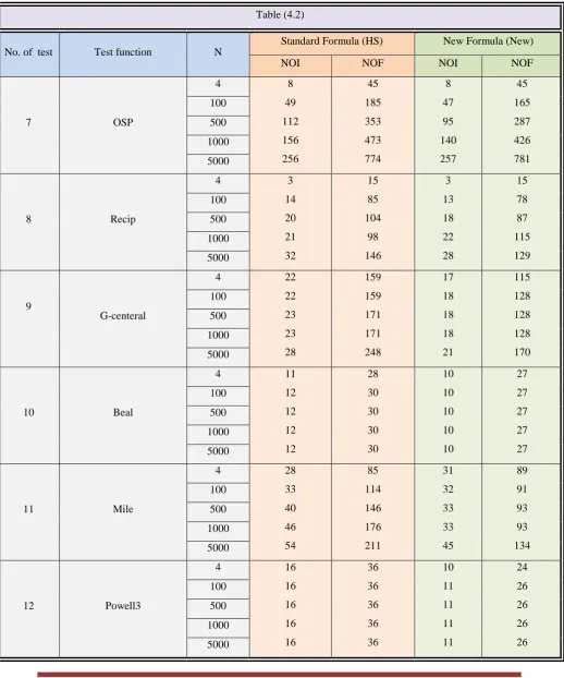
of function NOF. Experimental results in tables (4.1), (4.2) and (4.3) confirm that the new conjugate gradient

algorithm (New) is superior to standard algorithm (H/S)

Comparative Performance of Two Algorithm Standard

𝐇/𝐒

and New Formula

Table (4.1)

No. of test Test function N

Standard Formula (HS) New Formula (New)

NOI NOF NOI NOF

1

Rosen

4 27

27 27 27 27 74 74 74 74 74 17 18 18 18 18 44 46 46 46 46 100 500 1000 5000

2 Cubic

4 13

13 13 13 14 40 40 40 40 42 14 16 17 17 17 41 45 49 49 49 100 500 1000 5000

3 Powell

4 38

40 41 41 41 108 122 124 124 124 35 36 36 36 37 87 89 89 89 91 100 500 1000 5000

4 Wolfe

4 17

49 52 70 170 35 99 105 141 349 10 47 55 56 130 21 95 111 113 274 100 500 1000 5000 5 Wood

4 26

27 28 28 28 59 61 63 63 63 26 26 26 26 30 57 57 57 57 65 100 500 1000 5000

6 Non-diagonal

4 24

Table (4.2)

No. of test Test function N

Standard Formula (HS) New Formula (New)

NOI NOF NOI NOF

7 OSP

4 8

49 112 156 256 45 185 353 473 774 8 47 95 140 257 45 165 287 426 781 100 500 1000 5000

8 Recip

4 3

14 20 21 32 15 85 104 98 146 3 13 18 22 28 15 78 87 115 129 100 500 1000 5000 9 G-centeral

4 22

22 23 23 28 159 159 171 171 248 17 18 18 18 21 115 128 128 128 170 100 500 1000 5000

10 Beal

4 11

12 12 12 12 28 30 30 30 30 10 10 10 10 10 27 27 27 27 27 100 500 1000 5000

11 Mile

4 28

33 40 46 54 85 114 146 176 211 31 32 33 33 45 89 91 93 93 134 100 500 1000 5000

12 Powell3

4 16

Comparing the rate of improvement between the new algorithm (New) and the standard

algorithm (H/S)

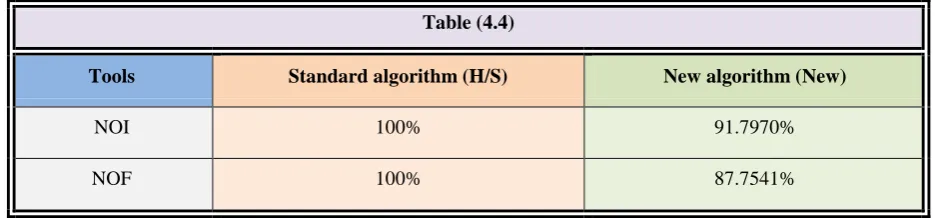
Table (4.4) shows the rate of improvement in the new algorithm (New) with the standard algorithm (H/S), The numerical results of the new algorithm is better than the standard algorithm, As we notice that (NOI), (NOF) of the standard algorithm are about 100%, That means the new algorithm has improvement on standard algorithm prorate (8.203%) in (NOI) and prorate (12.2459%) in (NOF), In general the new algorithm (New) has been improved prorate (10.22445%) compared with standard algorithm (H/S).

Table (4.3)

No. of test Test function N

Standard Formula (HS) New Formula (New)

NOI NOF NOI NOF

13 G-full

4 3

134

297

390

885

7

269

595

781

1771

3

117

273

388

885

7

235

547

777

1771 100

500

1000

5000

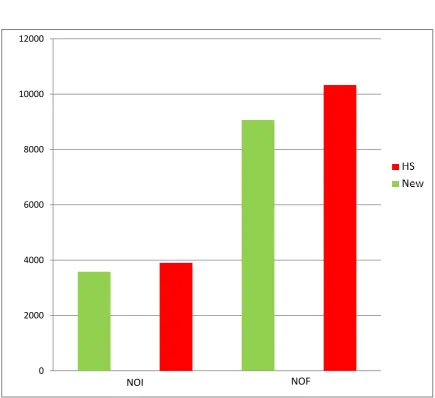
Total 3901 10330 3581 9065

Table (4.4)

Tools Standard algorithm (H/S) New algorithm (New)

NOI 100% 91.7970%

Figure (4.1) shows the comparison between new algorithm (New) and the standard algorithm (H/S) according to the total number of iterations (NOI) and the total number of functions (NOF).

V.

CONCLUSION

In this paper, we proposed a new and simple 𝛽𝑘𝑁𝑒𝑤 that has global convergence properties. Numerical results have shown that this new 𝛽𝑘𝑁𝑒𝑤performs better than Hestenes and E. Steifel (HS) . In the future we can we suggest formulas for 𝛾.

0 2000 4000 6000 8000 10000 12000

References

[1]. A. Abashar, M. Mamat, M. Rivaieand I. Mohd, Global Convergence Properties of a New Class of Conjugate Gradient Method for Unconstrained Optimization, International Journal of Mathematical Analysis, 8 (2014), 3307-3319.

[2]. AL - Bayati, A.Y. and AL-Assady, N.H.,Conjugate gradient method,Technical Research , 1 (1986), school of computer studies, Leeds University.

[3]. E. Polak and G. Ribiere, Note sur la convergence de directionsconjugees, Rev. FrancaiseInformatRechercheOperationelle. 3(16) (1969), pp. 35-43.

[4]. G. Zoutendijk, Nonlinear programming computational methods, Abadie J. (Ed.) Integer and nonlinear programming, (1970), 37-86.

[5]. M.R. Hestenes and E. Steifel, Method of conjugate gradient for solving linear equations, J. Res. Nat. Bur. Stand. 49 (1952), pp. 409-436

[6]. M. Rivaie, A. Abashar, M. Mamat and I. Mohd, The Convergence Properties of a New Type of Conjugate Gradient Methods, Applied Mathematical Sciences, 8 (2014),33-44.

[7]. M. Rivaie, M. Mamat, L. W. June and I. Mohd, A new conjugate gradient coefficient for large scale nonlinear unconstrained optimization, International Journal of Mathematical Analysis, 6 (2012), 1131-1146.

[8]. R. Fletcher, and C. Reeves, Function minimization by conjugate gradients, Comput. J. 7(1964), pp. 149-154.

[9]. R. Fletcher, Practical method of optimization, vol 1, unconstrained optimization, John Wiley & Sons, New York, 1987.

[10]. W.W. Hager, H. Zhang, A new conjugate gradient method with guaranteed descent and an efficient line search, SIAM Journal on Optimization,16 (2005) 170–192

[11]. Y. H. Dai and Y. Yuan, A note on the nonlinear conjugate gradient method, J. Compt. Appl. Math., 18(2002), 575-582..