A linear, stabilized, non-spatial iterative, partitioned time stepping method for the nonlinear Navier–Stokes/Navier–Stokes interaction model

(1)

R E S E A R C H

Open Access

A linear, stabilized, non-spatial iterative,

partitioned time stepping method for the

nonlinear Navier–Stokes/Navier–Stokes

interaction model

Jian Li

1*

_{, Pengzhan Huang}

2

_{, Jian Su}

3

_{and Zhangxin Chen}

4

*_{Correspondence:} [email protected]

1_{Department of Mathematics,}

School of Arts and Sciences, Shaanxi University of Science and Technology, Xian, P.R. China Full list of author information is available at the end of the article

Abstract

In this paper, a linear, stabilized, non-spatial iterative, partitioned time stepping method is developed and studied for the nonlinear Navier–Stokes/Navier–Stokes interaction. A backward Euler scheme is utilized for the temporal discretization while a linear Oseen scheme for the trilinear term is used to aﬀect the spatial discretization approximated by the equal order elements. Therefore, we only solve a linear Stokes problem without spatial iterative per time step for each individual domain. Then, the method exploits properties of the Navier–Stokes/Navier–Stokes system to establish the stability and convergence by rigorous analysis. Finally, numerical experiments are presented to show the performance of the proposed method.

MSC: 35Q10; 65N30; 76D05

Keywords: Partitioned time stepping methods; Fluid–ﬂuid interface; Navier–Stokes equations; Convergence; Numerical experiments

1 Introduction

The Navier–Stokes equations are useful because they describe the physics of many realistic problems of academic and industrial interest. They may be used to model weather, ocean currents, water flow, and many other phenomena. Many important applications need an accurate solution of multi-domain, multi-physics coupling of one fluid with another (e.g., the Navier–Stokes with the Navier–Stokes problems) [3,4,31,32]. The uncoupled meth-ods for two fluids are coupled through their shared interface by a rigid-lid coupling con-dition, i.e., no penetration and a slip with a friction condition allowing a jump in the tan-gential velocities across the shared interface [12]. Physics-based uncoupled methods are different from the traditional ones in the sense that they focus on decomposing different physical domains by directly using the given physical interface conditions, which is the key idea of the method proposed in this paper. Moreover, these methods allow existing highly optimized codes for each subproblem to be used in parallel as black boxes at each time step to solve the coupled problem.

Efficient stabilized finite element methods have been widely used in scientific computa-tion to achieve high accuracy for the Navier–Stokes equacomputa-tions approximated by the equal

(2)

order elements in practice. While these methods have been shown to be very successful, the theory ensuring their convergence and advantages for a coupled problem is still un-der development. Recently, some results have been obtained for partitioned time stepping methods for the fluid–fluid interaction by using the finite element methods [12,13,25]. In this paper, we shall follow the state-of-the-art convergence theory by using the geometric averaging at three time levels of the slip velocity at the interface to compute a friction co-efficient and further establish stability and convergence of the presented method for the coupled fluid–fluid model. We stress that the extension of the general convergence theory to the partitioned time stepping method for the Navier–Stokes/Navier–Stokes interaction is derived from that in [12]. Here, in order to ensure the balance between the spatial and temporal computing allocation, an unconditional stable backward Euler scheme is utilized for the temporal discretization while the linear Oseen scheme is applied for the trilinear term with a non-spatial iterative correction per time step. The method presented results in a better coefficient matrix of the form (aij)N×N=ν(∇φi,∇φj) + ((C· ∇)φi,φj), improving the model presented with small viscosity [16,17]. However, the difficulty for the numeri-cal analysis arises from the trilinear term and the whole system for the presented discrete finite element scheme.

The rest of paper is organized as follows. In Sect.2, we introduce the ﬂuid–ﬂuid model using two Navier–Stokes problems. In Sect.3, the stability of the Navier–Stokes/Navier– Stokes interaction model is analyzed. In Sect.4, the convergence of the presented method is analyzed. Finally, we present several numerical examples to illustrate the features of the proposed method in Sect.5.

2 Preliminary

A coupled Navier–Stokes/Navier–Stokes problem is stated as follows:

ui,t–νiui+ui· ∇ui+∇pi=fi inΩi, (1)

–νini· ∇ui·τ=k|ui–uj|(ui–uj)·τ onI, (2)

ui·ni= 0 onI, (3)

∇ ·ui= 0 inΩi, (4)

ui(x, 0) =u0i(x) inΩi, (5)

ui= 0 onΓi=∂Ωi\I. (6)

Here,i,j= 1, 2,i=j. Let the domainΩ=Ω1∪Ω2consist of two subdomainsΩ1andΩ2of

Rd,d= 2, 3, with the outward unit normal vectorsn1andn2, respectively, coupled across

the interfaceI. The viscosityνi> 0, the body forcefi: [0,T]→H1(Ωi), and the parameter k∈Rare given,i= 1, 2. Also,ui:Ωi×[0,T]→Rdandpi:Ωi×[0,T]→Rrepresent velocity and pressure on the subdomainsΩi, respectively,i= 1, 2.

For the mathematical problem (1)–(6), the following Hilbert spaces are introduced [1]:

Xi=

vi∈

H1(Ωi)

d

:vi= 0 onΓiandvi·ni= 0 onI

,

Mi=

qi∈L2(Ωi) :

Ωi

qidx= 0

(3)

Multiplying (1) byvi∈Xiand (4) byqi∈Mi, integrating and applying the divergence the-orem, the above coupled problem is equivalent to ﬁnding (ui,pi)∈(Xi,Mi) such that

(ui,t,vi) +a(ui,vi) –d(vi,pi) +b(ui,ui,vi) +κ

I

[u] [u]vids= (fi,vi),

d(ui,qi) = 0, ∀(vi,qi)∈(Xi,Mi),

(7)

where [·] denotes the jump of the indicated quantity across the interfaceI: [u] =ui–uj and

(ui,t,vi) =

Ωi

∂ui

∂t vidx, i= 1, 2.

The continuous bilinear formsa(·,·) andd(·,·) are deﬁned onXi×XiandXi×Mi, respec-tively, by

a(ui,vi) =νi(∇ui,∇vi), ui,vi∈Xi,

d(vi,qi) = –(vi,∇qi) = (divvi,qi), vi∈Xi,qi∈Mi.

These bilinear terms satisfy the following continuity andinf–supproperties:

a(ui,vi) ≤ν ∇ui 0 ∇vi 0,

d(vi,pi) ≤C ∇vi 0 pi 0,

sup

vi∈Xi

|d(vi,qi)

∇vi 0 ≥

β qi 0 ∀qi∈Mi,β> 0,

(8)

where the positive constantsCandβonly depend onΩ. Similarly, by using the divergence theorem, (3) and (6), the trilinear termb(·,·,·) can be deﬁned as follows [36]:

b(ui,vi,wi) = 1

2(ui· ∇vi,wi) + 1 2

(divui)vi,wi

=1

2(ui· ∇vi,wi) – 1

2(ui· ∇wi,vi), ui,vi,wi∈Xi. (9)

Obviously, the trilinear termb(·,·,·) satisﬁes the following skew-symmetry property [36]:

b(ui,vi,wi) = –b(ui,wi,vi).

A realistic model would contain many more complex terms. Here, we mainly focus on an algorithmic issue so we assume that the solution of (1)–(6) to be approximated is a strong solution. Moreover, the energetic stability of the monolithic problem is valid:

2

i=1

1 2

d dt ui

2

0+νi ∇ui 20

+κ

I

_[u] 3

ds=

2

i=1

(4)

3 Stabilizations for Galerkin approximations

Given a respective shape-regular and conforming triangulationThi ofΩi, the ﬁnite

ele-ment method is to solve (7) in two pairs of ﬁnite dimensional spaces (Xh

i,Mhi)⊂(Xi,Mi) [9,11,15,36].

Stabilization of the Stokes’ problem using local pressure projections dates back to the papers of Silvester [33,34], Brecker and Braack [2], Brezzi and Fortin [6], Brezzi and Pitki-ranta [7], Dohrmann and Bochev [14], Connors [23] and [8]. They provide a wide theoret-ical framework for these methods. The aim of the section is to give an elementary applica-tion in the spirit of these papers for a class of pressure projecapplica-tion method with equal order distribution for both velocity and pressure, which are computationally convenient and ef-ficient in a parallel and multigrid context. Then, the unstable velocity–pressure pairs of the equal-order finite elements are defined as follows [22,26–29,38]:

X_ih=vh∈X:vh|K∈

Rr(K)

d

,∀K∈Kh

,

Mh_i =qh∈M:qh|K∈Rr(K),∀K∈Kh

, r= 1, 2.

In order to analyze the stabilzation of the Galerkin approximations for the Navier– Stokes/Navier–Stokes interaction, we assume thatπ_ihdenotes the interpolation operator from the richer spaceMhinto the smaller spaceM¯h⊂Mhsuch thatXh× ¯Mhsatisﬁes the inf–sup condition anddivXh⊂Mh.

Lemma 3.1 It holds that

sup

vh_i∈X_ih d(vh

i,qhi)

∇vh i 0

+G1/2qh_i,qh_i≥β0qhi0, q

h i ∈Mih,

where the positive constantβ0only depends onΩand the stabilized term G(·,·)is deﬁned

as follows:

Gqh_i,qh_i∼

⎧ ⎨ ⎩

qh

i –πiqhi0, r= 1,

_h_∇

qh_i –πiqhi0, r= 2.

(11)

Proof For a bounded Lipschitz connected domainΩand for anyph_i ∈L2(Ω), there exist a positive constantC0> 0 andvi∈[H1(Ωi)]dsatisfying

divvi=phi

such that

vi 1≤C0phi0

and

ph_i2₀=dvi,phi

(5)

Then, there exists a linear operatorπ˜_ih: [H1₍_Ω

i)]d→Xhsuch that the orthogonality rela-tion holds [5,10]:

vi–π˜ihvi,qh

= 0, ∀qh∈Mh, (12)

_{∇ ˜}π_ihvi₀≤C vi 1≤C1phi0, (13)

whereC1only depends onΩ. Noting thatdivπ˜hv∈Mhand thusd(π˜hv,phi –πhphi) = 0, and using the deﬁnition ofπ˜h, we obtain

ph_i2₀=dvi,phi

=dvi,phi –πihphi

+dvi,πihphi

=dvi–π˜hvi,phi –πihphi

+dπ˜hvi,πihphi

=dvi–π˜hvi,phi –πihphi

+dπ˜_ihvi,phi

, (14)

where

dvi–π˜ihvi,phi –πihphi

≤Cph_i –π_ihph_i₀ vi 1

≤G1/2ph_i,p_ihph_i₀, r= 1, (15)

and

dvi–π˜ihvi,phi –πihphi

= –∇ph_i –π_ihph_i,vi–π˜ihvi

≤Ch∇ph_i –π_ihph_i₀ vi 1

≤G1/2ph_i,p_ihph_i₀, r= 2.

Therefore,

sup

vh_i∈X_ih

d(vh_i,qh_i)

∇vh_i 0 +G

1/2_ph i,phi

≥ d(π˜ivi,qhi)

∇ ˜πivi 0

+G1/2ph_i,ph_i

≥β0phi

2 0.

For more details, the result related to the well-posedness of the Navier–Stokes/Navier– Stokes interaction can be found in [12,13,18,20,30,37].

4 Stability

In this section, we are now in a position to state a discrete ﬁnite element scheme. We let (un

i,pni) =: (uni,h,pni,h),i= 1, 2, denote a discrete approximation toui(tn), where the discrete timetn_{is calculated from the uniform time step size}_τ ₌_T_/N_by_tn₌_n_τ_,_n_{= 0, 1, . . . ,N.}

From the point of view of implementation, the method presented consists of several subroutines for solving the nonlinear fluid–fluid interaction. First, the first guessu0

(6)

un_i+1,n= 0, 1, 2, . . . , can be obtained by the following equations (16) and (17). For the nu-merical treatment of the time derivative term, we use the fully discrete backward Euler ap-proximation. As for the partitioned scheme, we apply the Oseen scheme with a non-spatial iterative correction to simplify the trilinear term per time step and further obtain a better stiﬀness matrix. Especially, recalling the standard geometric averaging of the jump in [12,

The linear, stabilized, non-spatial iterative, partitioned time stepping method is deﬁned as follows:

Step I.Find(u1

i,p1i)∈Xih×Mihsatisfying the followingStokesequations:

au1_i,vi

–dvi,p1i

+du1_i,qi

+Gp1_i,qi

= (f,vi) ∀(vi,qi)∈Xih×Mhi.

Moreover, set the iterative stepm= 1, 2, . . . , the error of two successive solutions

em_i =um_i –um_i –12+pm_i –pm_i –12<ε

with a suﬃciently small iterative toleranceε> 0.

Step II.Solve the Navier–Stokes/Navier–Stokes interaction: Givenτ> 0,fi∈[H–1(Ωi)]d (i= 1, 2),ﬁnd(un₁+1,p₁n+1)∈Xh₁×M₁hsuch that

(un+1

1 –un1,v1)

τ +a

un₁+1,v1

–dv1,pn1+1

+dun₁+1,q1

+Gpn₁+1,q1

+b1

un₁,un₁+1,v1

+k

I

un un₁+1v1ds–k

I

un 1/2 un–1 1/2un₂·v1ds

=f1

tn+1,v1

, ∀(v1,q1)∈X1h×M1h, (16)

and(un₂+1,pn₂+1)∈X₂h×Mh₂such that

(un₂+1–un₂,v2)

τ +a

un₂+1,v2

–dv2,pn2+1

+dun₂+1,q2

+Gpn₂+1,q2

+b2

un₂,un₂+1,v2

+k

I

un un₂+1v2ds–k

I

un 1/2 un–1 1/2un₁·v2ds

=f2

tn+1,v2

∀(v2,q2)∈X2h×Mh2. (17)

This, of course, dictates that the overall structure of the linear, stablized, non-spatial iterative, partition time step method will be much the same as for a standard ﬁnite el-ement method, as described in [12]. The key point of the presented method is to use a linear, non-spatial iterative, partitioned time stepping method for the nonlinear Navier– Stokes/Navier–Stokes interaction model.

Routine: [u0

(7)

[um_h,pm_h] = LNS(Th,umh–1,f); end while

end for

In this section, we aim to establish a result concerning the unconditional stability of the scheme (16)–(17).

Lemma 4.1 Let un_i,i= 1, 2,n= 1, 2, . . . ,m,be the solutions of equations(16)and(17).Then we have the following energy inequality:

um+12

0+

m

n=1

un+1– un2₀+τ

m

n=1

ν1∇un1+1 2

0+ν2∇u

n+1

2

2 0

+κτ

I

un un₁+1 2+ un₂+1 2ds

≤u12₀+κτ

I

u0 u1₁ 2+ u1₂ 2ds

+ m

n=1

τ ν1

f1

tn+12₀+ τ

ν2

f2

tn+12_–1

, (18)

where un

i = (un1,un2)with the norm un 0= (

2

i=1 uni 20)1/2.

Proof Noting that

bun_i,u_in+1,un_i+1= 0,

we start by testing (16) and (17) with (vi,qi) = 2(τuni+1,pni+1), respectively, to obtain 2un_i+1–un_i,u_in+1+ 2νiτ∇uni+1

2 0+ 2G

pn_i+1,pn_i+1

+ 2κτ

I

un_i+1 2 un ds–

I

un 1/2 un–1 1/2un_i₊₁·un_i+1ds

= 2τfi

tn+1,un_i+1 ∀(vi,qi)∈Xih×Mhi,i= 1, 2, (19)

whereu3=u1when the index is out of bounds. Using the identity

2(a–b,a) =a2+ (a–b)2–b2, (20)

and combing with (19) withi= 1, 2, we obtain the following result:

un+12

0–u

n2 0+u

n+1_{– u}n2

0+ 2ν1τ∇u

n+1

1

2

0+ 2ν2τ∇u

n+1

2

2 0

+ 2κτ

2

i=1

I

_un+1

i

2

un ds–

I

un 1/2 un–1 1/2un_i₊₁·un_i+1ds

+ 2Gpn_i+1,pn_i+1

= 2τ

2

i=1

fi

(8)

where

κ

I

un_i+1 2 un ds–

I

un 1/2 un–1 1/2un_i₊₁·un_i+1ds

=κ 2

I

un_i+1 2 un ds–κ 2

I

un_i₊₁ 2 un–1 ds

+κ 2

I

un_i+1 un 1/2–un_i₊₁ un–1 1/2 2ds,

2τ 2 i=1 fi

tn+1,un_i+1

≤2τ γ

2

i=1

fi

tn+1₀∇un_i+1₀

≤ 2

i=1

τ νi∇uni+1

2 0+

τ γ2 νi

fi

tn+12₀

,

(22)

where the positive constant is derived from the Poincaré inequality. Then, substituting these into (21), we infer that

un+12₀–un2₀+un+1– un2₀+ν1τ∇un1+1 2

0+ν2τ∇u

n+1 2 2 0 +κτ I

un₁+1 2+ u₂n+1 2 un ds–κτ

I

un₁ 2+ un₂ 2 un–1 ds

+κτ

2

i=1

un+1

i un

1/2

–un

i+1 un–1 1/2 2

ds

≤τ

2

i=1

fi(tn+1) 20

νi

. (23)

Summing overn= 1, 2, . . . ,myields the desired result.

5 Convergence

In this section, we consider the convergence of the presented method for the Navier– Stokes/Navier–Stokes interaction. First, we provide the discrete Gronwall’s inequality [21,

24], which will be useful in the subsequent analysis.

Letan+1_,_bn+1_,_cn+1_,_dn+1_and_Dn+1_,_n_{= 0, 1, 2, . . . ,}_{m, be ﬁve nonnegative sequences}

satis-fying

am+1+ m

n=0

bn+1+τ

m

n=0

cn+1≤C1+C2τ

m

n=0

Dn+1an+1+C3τ

m

n=0

dn+1. (24)

Then we have the following result:

am+1+ m

n=0

bn+1+τ

m

n=0

cn+1≤exp

C2τ

m

n=0

σn+1

C1+C3τ

m

n=0

dn+1

(9)

where

σn+1= D n+1

1 –τDn+1.

In order to analyze convergence of the partitioned time stepping methods for the fluid–fluid interaction, we introduce the following Stokes projection by finding (Rh(vi,qi), Qh(vi,qi))∈Xih×Mhi such that

avi–Rh(vi,qi),vh

–dvh,qi–Qh(vi,qi)

+dvi–Rh(vi,qi),qh

= 0,

(vh,qh)∈Xih×Mhi, (26)

which is well-deﬁned and satisﬁes the following optimal approximation property:

vi–Rh(vi,qi)₀+h∇

vi–Rh(vi,qi)₀+qi–Qh(vi,qi)₀

≤Ch2 vi 2+ qi 1

, i= 1, 2. (27)

Theorem 5.1 Assume that the initial data u0

i and u1i satisfy the following estimate:

_∇

ui

t0–u0_i₀+∇ui

t1–u1_i₀≤Ch, i= 1, 2. (28)

Moreover,the time stepτ satisﬁes the relationτ < 1/Dn+1_{with D}n+1 _{deﬁned by}₍₄₃₎

be-low. Let (ui,pi) and (uni+1,pin+1)be the solutions of (1)–(6) and(16)–(17), respectively, with ui∈L2([0,T],H2(Ωi)∩Xi),pi∈L2([0,T],H1(Ωi)∩Mi),ui,t∈L2([0,T],Xi)and ui,tt∈ L2_([0,_T],_L2₍_Ω

i)).Then it holds that

τ

m

n=0

ν1∇

u1

tn+1–u₁n+12₀+ν2∇

u2

tn+1–un₂+12₀

≤Cτ2+h2r, r= 1, 2, (29)

where C denotes a positive constant depending on the data(νi,Ωi,ui,pi,fi),i= 1, 2,which may stand for diﬀerent values at diﬀerent occurrences.

Proof Here, we analyze convergence on each subdomain independently. For convenience, we set (ej_i,η_ij) = (Rhui(tj) –uji,Qhpi(tj) –pji) andE

j

i=ui(tj) –Rhui(tj). First, using the Stokes projection, we subtract (16) or (17) from (7) with (vi,qi) = (eni+1,ηni+1)∈Xih×Mihto obtain

∂ui(tn+1)

∂t –

(un+1

i –uni)

τ ,e

n+1

i

+aen_i+1,en_i+1+ 2Gηn_i+1,ηn_i+1

+bui

tn+1,ui

tn+1,en_i+1–bun_i,un_i+1,en_i+1

+κ

I ui

tn+1 utn+1 ·en_i+1ds–

I

un_i+1 un ·en_i+1ds

+κ

I

un_j un 1/2 un–1 1/2·en_i+1ds–

I uj

tn+1 utn+1 ·en_i+1ds

= 2Gpi

tj+1,ηi

(10)

wherei= 1,j= 2 ori= 2,j= 1. We analyze each term in the above equality. Note that

∂ui(tn+1)

∂t –

(un_i+1–un_i)

τ ,e

n+1

i

=1

τ

ui

tn+1–un_i+1–ui

tn–un_i,en_i+1–1

τ

ui

tn+1–ui

tn,en_i+1

+

∂ui(tn+1)

∂t ,e n+1

i

=1

τ

En_i+1–E_in,en_i+1+1

τ

en_i+1–en_i,en_i+1–RHSn_i+1,en_i+1,

where (RHSn+1

i ,v) = (ui

(tn+1)–ui(tn)

τ –

∂ui(tn+1)

∂t ,vi),i= 1, 2. Also, we see that

_En+1

i –Eni,eni+1 ≤ 1 4ε1νi

_En+1

i –Eni

2

–1+ε1νi∇e

n+1

i

2

0, (31)

RHSi,eni+1 ≤ 1 4ε2νi

RHS_in+12_–1+ε2νi∇eni+1

2

0, (32)

whereεi> 0,i= 1, 2. For the trilinear terms, it is easy to see that

bui

tn+1,ui

tn+1,en_i+1–bun_i,un_i+1,en_i+1

=bui

tn+1–ui

tn,ui

tn+1,en_i+1+bEn_i,ui

tn+1,en_i+1

+ben_i,ui

tn+1,en_i+1–bun_i,ui

tn+1–un_i+1,en_i+1

=I1+I2+I3+I4. (33)

To estimate these trilinear terms, using a classical result in [36], we see that

|I1| ≤C∇ui

tn+1–ui

tn₀∇ui

tn+1₀∇en_i+1₀

≤ε3νi∇eni+1

2 0+

C 4ε3νi

_∇ui

tn+12₀∇ui

tn+1–ui

tn2₀.

Applying the Young inequality and the skew-symmetry of the trilinear term yields that

|I2+I4|= b

E_in,ui

tn+1,en_i+1–bun_i,En_i+1,en_i+1

≤∇un_i₀+∇ui

tn+1₀∇En_i₀+∇En_i+1₀∇en_i+1₀

≤ε4νi∇eni+1

2 0+

c 4ε4νi

_∇_un i

2 0+∇ui

tn+12₀En_i₀2+En_i+12₀.

For the third termI3, using the following inequality [20]:

φ _L4≤C φ 1 2–14(d–2)

0 ∇φ

1 2+14(d–2)

(11)

and applying the Young inequality and the Cauchy–Schwarz inequality, we have

|I3| ≤Cen_i1/2₀ ∇en_i1/2₀ ∇ui

tn+1₀∇en_i+1₀

≤ε5νi∇eni+1

2 0+Ce

n i0∇e

n i0∇ui

tn+12₀

≤ε5νi∇eni+1

2

0+ε6νi∇e

n i

2 0+Ce

n i

2 0∇ui

tn+14₀

ford= 2, and

|I3| ≤Cen_i1/4₀ ∇en_i3/4₀ ∇ui

tn+1₀∇en_i+1₀

≤ε5νi∇eni+1

2 0+Ce

n i

1/2 0 ∇e

n i

3/2 0 ∇ui

tn+12₀

≤ε5νi∇eni+1

2

0+ε6νi∇e

n i

2 0+Ce

n i

2 0∇ui

tn+18₀

ford= 3. Setting

utn+1 ₌1

2 u

tn+1 + utn ,

un ₌1 2 u

n ₊ _un–1 _,

and using the same approach as in [12], we get

I5 =

I ui

tn+1 utn+1 ·en_i+1ds–

I

un_i+1 un ·en_i+1ds

=

I ui

tn+1 utn+1 – utn ·en_i+1ds

+

I ui

tn+1 utn – Phu

tn ·en_i+1ds

+

I ui

tn+1 Phu

tn – un ·en_i+1ds

+

I

E_in+1 un ·en_i+1ds+

I

un en_i+1 2ds

≤

I ui

tn+1 _u_tn+1 _– _u_tn _·_en+1

i ds+

I ui

tn+1 _En i ·en

+1 i ds + I ui

tn+1 en_i ·en_i+1ds

+

I

E_in+1 un ·en_i+1ds+

I

un en_i+1 2ds. (35)

Noting that

utn _– _u_tn+1

=1 2 u

tn – utn+1 +1 2 u

tn–1 – utn+1

≤1

2 u

(12)

and

un 1/2 un–1 1/2– un _|

=1 2 u

n 1/2_– _un–1 1/22

≤1

2 u

n _– _un–1

≤1

2 u

n_{– u}n–1

≤1

2 u

n_{– u}_tn_{+ u}_tn–1_{– u}n–1 ₊1

2 u

tn– utn–1

≤ en ₊ _En ₊ _en–1₊_En–1 ₊1

2 u

tn– utn–1 , (37)

the following error bound holds:

I6 =

I

un_j un 1/2 un–1 1/2·en_i+1ds–

I uj

≤

I

un_j un 1/2 un–1 1/2– un _·_en+1

i ds+

I

un_j un _–_P

h un ·eni+1ds

+

I

un_jPh un – u

tn ·en_i+1ds

+

I

un_j utn+1 _– _u_tn+1 _·_en+1

i ds

–

I

En_j +en_j utn+1 ·en_i+1ds

+

I

uj

tn–uj

≤

I

un_j utn– utn–1 ·en_i+1ds+

I

un_j En _·_en+1

i ds+

I

un_j en _·_en+1

i ds

+

I

un_j utn– utn+1 + utn–1– utn+1 ·en_i+1ds

+

I

uj

tn–uj

–

I

En_j +en_j utn+1 ·en_i+1ds. (38)

Applying the same approach as in [12], we obtain

|I5+I6|

≤ε7νi∇eni+1

2 0+Cν

–3

i

1 +un₂4_I +utn+14_Ien_i+12₀

+ε8 2

i=1

νi∇eni

2 0+∇e

n–1

i

2 0

+CLn+1Pn+1

+CMn+1

2

i=1

(13)

whereLn+1_,_Mn+1_and_Pn+1_{can be deﬁned by the following bound terms on interface}_I_as

follows:

Ln+1₌ 2

i=1

ui

tn+12

I +u n+1

i

2

I +u n i 2 I ,

Mn+1=

2

i=1

_u_i

tn+14_I +un_i4_I,

Pn+1=

2

i=1

ui

tn+1–ui

tn2_I +ui

tn+1–ui

tn–12_I

+E_in–12_I +En_i2_I +En_i+12_I.

Obviously, · I is bounded by the correspondingL2-norm. In addition, we can infer that the estimate ofPn+1_{has the order of}_O(_τ2₊_h2r_),_r_{= 1, 2.}

Choosingε1+ε2+ε3+ε4+ε5+ε7= 1/4,ε6= 1/8, andε8= 1/16, and combining all these

inequalities with (30) yields that 1

2τe

n+1

i

2 0–e

n i

2 0+e

n+1

i –eni

2 0

+3νi 4 ∇e

n+1 i 2 0 ≤C 1

τE

n+1

i –Eni

2

–1+RHS

n+1

i

2

–1+ pi–Πhpi 2 0

+C∇ui

tn+12₀∇ui

tn+1–ui

tn2₀

+∇un_i2₀+∇ui

tn+12₀En_i2₀+E_in+12₀+Cen_i2₀∇ui

tn+12₀d

+Cν_i–31 +un₂4_I +utn+14_Ien_i+12₀+CLn+1Pn+1

+

2

i=1

νi 16∇e

n i

2 0+∇e

n–1

i

2 0

+νi 8∇e

n i

2 0

+CMn+1

2

i=1

ν_i–3en_i2₀+en_i–12₀. (40)

Summing overi= 1, 2 for the above inequality and moving the term on the 5th line on the right-hand side of (40) to its left-hand side, t the term νi

8 ∇e

n

i 20can be exactly absorbed.

Thus we ﬁnd that

1 2τe

n+12 0–e

n2 0+e

n+1_{– e}n2 0 + 2 i=1 νi 2∇e

n+1 i 2 0 + 2 i=1 νi 4∇e

n+1

i

2 0–∇e

n i 2 0 + 2 i=1 νi 16∇e

n i

2 0–∇e

n–1 i 2 0 ≤C 2 i=1 1

τE

n+1

i –Eni

2

–1+RHS

n+1

i

2

–1+ pi–Πhpi 2 0 +C 2 i=1

_∇ui

tn+12₀∇ui

tn+1–ui

(14)

+C

2

i=1

_∇_un i

2 0+∇ui

tn+12₀En_i₀2+En_i+12₀+C

2

i=1

Ln+1Pn+1

+C

2

i=1

ν_i–31 +un₂4_I +utn+14_Ien_i+12₀+C

2

i=1

en_i2₀∇ui

tn+12₀d

+C

2

i=1

ν_i–3Mn+1en_i₀2+en_i–12₀.

Noting the bounds of ∇ui(tn+1) 0,

m–1

n=0 ∇uni+1 0, and utt 0yields

E_in+1–E_in_–12 +τRHSn_i+12_–1

≤Cτ2+h2 utt 2_L2_([_t

n–1,tn+1],L2(Ωi))

+ u _L2_([_t

n–1,tn+1],H2(Ωi))+ p L2([tn–1,tn+1],H1(Ωi))

,

Ln+1Pn+1

≤Cτ2+h2r ut 2_L2_([_t_n_–1_,_t_n₊₁_],_L2₍_Ω

i))+ u

2

L2_([_t_n_–1_,_t_n₊₁_],_H2₍_Ω

i))

.

Summing over n= 1, 2, . . . ,m– 1, multiplying by 2τ, using the classical estimates, and rewritting the last term of the right-hand side of the above inequality as

m–1

n=1

₂

i=1

ν_i–3Mn+1en_i2₀+en_i–12₀

≤C

2

i=1

ν_i–3M2+M3e1_i2₀+e0_i2₀+C m–1

n=1

ν_i–3Mn+1+Mn+2en2₀, (41)

we obtain

em2

0+

m–1

n=1

en+1– en2₀+τ

m–1

n=1 2

i=1

νi 2∇e

n+1

i

2 0

+τ

2

i=1

νi 16∇e

m–1

i

2 0+ 4∇e

m i

2 0

≤τ

2

i=1

νi 16∇e

0

i

2 0+ 4∇e

1

i

2 0

+1 +Cτ ν_i–3M2+M3e02₀+e12₀

+Cτ2+h2r+Cτ

m–1

n=1

Dn+1en+12

0, (42)

whereDn+1_{is deﬁned by}

Dn+1=ν_i–31 +Mn+Mn+1+un₂4_I +utn+14_I

(15)

andCis dependent of the data (Ωi,νi,fi). Setting

aj+1=ej+12₀, bj+1=ej+1–ej2₀, cj+1=

2

i=1

_∇ej_i+12₀,

and using Gronwall’s inequality in Lemma4.1, (28) and (42) yields the desired result.

6 Numerical results

In this section, we assess numerical performance of the stabilized methods for the pre-sented model. It will be checked by a known analytical solution problem. The main goal of the experiment is to verify convergence rates of the scheme (16)–(17). Here, we denote errors by

Err(ui) =

τ

m

n=0

_∇

ui

tn+1–un_i+12_0,_Ω

i

1/2

,

Err(pi) =

τ

m

n=0

pi

tn+1–pn_i+12_0,_Ω

i

1/2

,

where i= 1, 2. All numerical computations are implemented by open source software Freefem [19].

Example1 The computations of the experiment are carried out in the domains Ω1=

(0, 1)×(0, 1) andΩ2= (0, 1)×(–1, 0). The prescribed exact solutions are given [13,37]

by

p1(t,x,y) =p2(t,x,y) =exp(–t)cos(πx)sin(πy),

u1,1(t,x,y) = –αx2exp(–t)(x– 1)2(y– 1),

u1,2(t,x,y) =αxyexp(–t)

6x+y– 3xy+ 2x2y– 4x2– 2,

u2,1(t,x,y) = –αxexp(–t)(x– 1)

y2x(x– 1)

μ1

μ2

+ 1

–μ

1/2

1 y2exp(t/2)

(ακ)1/2 –x(x– 1) +

μ1/2₁ exp(t/2) (ακ)1/2 +

μ1xy(x– 1)

μ2

,

u2,2(t,x,y) = –

αyexp(–t)(2x– 1) 3μ2(ακ)1/2

6μ2x2(ακ)1/2– 6μ2x(ακ)1/2– 3μ1/21 μ2exp(t/2)

– 2μ1x2y2(ακ)1/2– 2μ2x2y2(ακ)1/2+ 3μ1xy(ακ)1/2+ 2μ1xy2(ακ)1/2

– 3μ1x2y(ακ)1/2+ 2μ2xy2(ακ)1/2+μ1/21 μ2y2exp(t/2)

,

with an arbitrary positive constantα. Here, (ui,pi),i= 1, 2 are the solutions of the original problem (1)–(6) and the right-hand sidesf = (f1,f2) can be obtained by (1). Moreover,

u2= (u2,1,u2,2) satisﬁes the three interface conditions in [13].

Firstly, in the ﬁrst example, we choose the same parameter valuesμ1= 0.5,μ2= 0.05,

(16)

Table 1 Errors for stabilizedP1–P1pair withτ=h

1/h Err(u1) Rate Err(u2) Rate Err(p1) Rate Err(p2) Rate

8 7.2271E–2 – 2.9717E–1 – 1.4967E–2 – 1.1617E–2 –

32 1.7025E–2 1.043 7.0463E–2 1.038 1.8549E–3 1.506 1.9019E–3 1.305 64 8.4129E–3 1.017 3.4862E–2 1.015 6.8180E–4 1.444 7.2067E–4 1.400

Table 2 Errors for stabilizedP2–P2pair withτ=h2

1/h Err(u1) Rate Err(u2) Rate Err(p1) Rate Err(p2) Rate

4 2.6926E–2 – 1.7999E–1 – 1.7270E–2 – 1.6852E–2 –

8 5.7926E–3 2.215 3.4207E–2 2.396 4.2766E–3 2.014 4.2613E–3 1.984 16 1.3445E–3 2.107 6.9341E–3 2.303 1.0623E–3 2.009 1.1131E–3 1.914

Table 3 Errors for the diﬀerent small viscosities based on stabilizedP1–P1pair

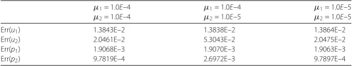
μ1= 1.0E–4 μ1= 1.0E–4 μ1= 1.0E–5

μ2= 1.0E–4 μ2= 1.0E–5 μ2= 1.0E–5

Err(u1) 1.3843E–2 1.3838E–2 1.3864E–2

Err(u2) 2.0461E–2 5.3043E–2 2.0475E–2

Err(p1) 1.9068E–3 1.9070E–3 1.9063E–3

Err(p2) 9.7819E–4 2.6972E–3 9.7897E–4

Table 4 Errors for the diﬀerent small viscosities based on stabilizedP2–P2pair

μ1= 1.0E– 4 μ1= 1.0E– 4 μ1= 1.0E– 5

μ2= 1.0E– 4 μ2= 1.0E– 5 μ2= 1.0E– 5

Err(u1) 4.9393E–2 4.9283E–2 5.4135E–2

Err(u2) 4.9196E–2 5.3924E–2 5.3904E–2

Err(p1) 3.0189E–4 3.0190E–4 3.0190E–4

Err(p2) 3.1022E–4 7.7659E–4 3.1042E–4

with the time step τ =h. Three values of space sizeh= 1/8, 1/32, 1/64 are chosen. We display the convergence orders and errors of the presented method in Tables1–2byPr– Pr,r= 1, 2. From Tables1–2, it can be easily seen that the method completely agree with the expected results in theory.

Secondly, we test the presented method with small viscosities. Here, we chooseα= 1,

κ = 100,h= 1/20 and the time stepτ = 0.005. Then, we list the numerical errors with diﬀerent small viscosities atT= 0.1 in Tables3–4. Obviously, the presented method can deal with these problems involving small viscosities.

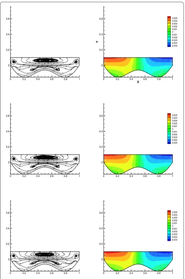
Example2 In this example, we test the presented method for a submarine mountain prob-lem. This problem describes the ﬂuid, which ﬂows in a domain including the submarine mountain. In this case, the subdomainΩ2is nonconvex. As is known, the viscosity of the

ﬂuid at submarine location is bigger than that at surface location. So we takeμ1= 0.001

andμ2= 0.01 in this example.

SetΩ1= [0, 1]×[0, 0.1] andΩ2={(x,y) :₄₀7(1 – (2x– 1)sin(7x– 3.5))≤y≤0}. The initial

conditions are chosen as follows:

p1(0,x,y) =p2(0,x,y) =cos(πx)sin(πy),

(17)

Figure 1The numerical streamlines and isobars: the stabilizedP2–P2pair (the ﬁrst line), theP2–P1pair (the second line) and the stabilizedP1–P1pair (the third line)

u1,2(0,x,y) =xy

–0.2 +y+ 0.6x– 3xy– 0.4x2+ 2x2y,

u2,1(0,x,y) =x2(1 –x)2(0.1 +y),

u2,2(0,x,y) =xy

(18)

We apply the presented method to get the numerical solution withh= 1/70 andτ= 1/40. In Fig.1, we present profiles for the numerical velocity and pressure with different methods at the final timeT= 5 andκ= 100. From this figure, we can see that the stabilized methods are stable and the unphysical oscillations do not appear, and the numerical results of these stabilized methods completely agreement with those obtained by the classicalP2–P1pair

[35]. Besides, we can find that the presence of the submarine mountain affects the fluid.

Acknowledgements

The authors express their sincere thanks to the anonymous reviewers for their valuable suggestions and corrections for improving the quality of this paper.

Funding

This work is supported by NSF of China (No. 11771259 and 11861067).

Availability of data and materials

Data sharing not applicable to this article as no datasets were generated or analyzed during the current study.

Competing interests

The authors declare that they have no competing interests.

Authors’ contributions

All authors contributed equally to the writing of this paper. All authors read and approved the ﬁnal manuscript.

Author details

1_{Department of Mathematics, School of Arts and Sciences, Shaanxi University of Science and Technology, Xian, P.R. China.} 2_{College of Mathematics and System Sciences, Xinjiang University, Urumqi, China.}3_{School of Mathematics and Statistics,}

Xi’an Jiaotong University, Xi’an, P.R. China.4_{Department of Chemical & Petroleum Engineering, Schulich School of}

Engineering, University of Calgary, Calgary, Canada.

Publisher’s Note

Springer Nature remains neutral with regard to jurisdictional claims in published maps and institutional aﬃliations.

Received: 27 December 2018 Accepted: 4 June 2019

References

1. Adams, R.A.: Sobolev Spaces. Academic Press, New York (1975)

2. Becker, R., Braack, M.: A ﬁnite element pressure gradient stabilization for the Stokes equations based on local projections. Calcolo38, 173–199 (2001)

3. Bernardi, C., Chacón-Rebollo, T., Lewandowski, R., Murat, F.: Existence of a solution for a model of two coupled turbulent ﬂuids. SIAM J. Numer. Anal.40, 2368–2394 (2002)

4. Bresch, D., Koko, J.: Operator-splitting and Lagrange multiplier domain decomposition methods for numerical simulation of two coupled Navier–Stokes ﬂuids. Int. J. Appl. Math. Comput. Sci.16, 419–429 (2006)

5. Brezzi, F., Fortin, M.: Mixed and Hybrid Finite Element Methods. Springer, New York (1991)

6. Brezzi, F., Fortin, M.: A minimal stabilisation procedure for mixed ﬁnite element methods. Numer. Math.89, 457–491 (2001)

7. Brezzi, F., Pitkäranta, J.: On the stabilization of ﬁnite element approximations of the Stokes equations. In: Proceedings on the Eﬃcient Solutions of Elliptic Systems, Kiel, 1984. Notes on Numerical Fluid Mechanics, vol. 10, p. 11. Vieweg, Braunschweig (1984)

8. Burman, E.: Pressure projection stabilizations for Galerkin approximations of Stokes’ and Darcy’s problem. Numer. Methods Partial Diﬀer. Equ.24, 127–143 (2008)

9. Chen, Z.: Finite Element Methods and Their Applications. Springer, Heidelberg (2005)

10. Chen, Z., Wang, Z., Zhu, L., Li, J.: Analysis of the pressure projection stabilization method for the Darcy and coupled Darcy–Stokes ﬂows. Comput. Geosci.17, 1079–1091 (2013)

11. Ciarlet, P.G.: The Finite Element Method for Elliptic Problems. North-Holland, Amsterdam (1978)

12. Connors, J., Howell, J., Layton, W.: Decoupled time stepping methods for ﬂuid–ﬂuid interaction. SIAM J. Numer. Anal.

50, 1297–1319 (2012)

13. Connors, J.M., Howell, J.S.: A fluid–fluid interaction method using decoupled subproblems and differing time steps. Numer. Methods Partial Differ. Equ.28, 1283–1308 (2012)

14. Dohrmann, C.R., Bochev, P.B.: A stabilized ﬁnite element method for the Stokes problem based on polynomial pressure projections. Int. J. Numer. Methods Fluids46, 183–201 (2004)

15. Girault, V., Raviart, P.A.: Finite Element Method for Navier–Stokes Equations: Theory and Algorithms. Springer, Berlin (1987)

16. He, Y., Li, J.: Convergence of three iterative methods based on the ﬁnite element discretization for the stationary Navier–Stokes equations. Comput. Methods Appl. Mech. Eng.198, 1351–1359 (2009)

(19)

18. He, Y., Lin, Y., Sun, W.: Stabilized ﬁnite element method for the non-stationary Navier–Stokes problem. Discrete Contin. Dyn. Syst., Ser. B6, 41–68 (2006)

19. Hecht, F., LeHyaric, A., Pironneau, O.: Freefem++ version 3.23 (2013)http://www.freefem.org/ﬀ++

20. Heywood, J.G., Rannacher, R.: Finite-element approximations of the nonstationary Navier–Stokes problem. Part I: regularity of solutions and second-order spatial discretization. SIAM J. Numer. Anal.19, 275–311 (1982) 21. Heywood, J.G., Rannacher, R.: Finite-element approximation of the nonstationary Navier–Stokes problem part IV:

error analysis for second-order time discretization. SIAM J. Numer. Anal.27, 353–384 (1990)

22. Huang, P., Feng, X., He, Y.: A quadratic equal-order stabilized ﬁnite element method for the conduction–convection equations. Comput. Fluids86, 169–176 (2013)

23. Layton, W.: Model reduction by constraints, discretization of ﬂow problems and an induced pressure stabilization. Numer. Linear Algebra Appl.12, 547–562 (2005)

24. Layton, W.: Introduction to the Numerical Analysis of Incompressible Viscous Flows. Comput. Sci. Eng., vol. 6. SIAM, Philadelphia (2008)

25. Layton, W., Tran, H., Trenchea, C.: Analysis of long time stability and errors of two partitioned methods for uncoupling evolutionary groundwater–surface water ﬂows. SIAM J. Numer. Anal.51, 248–272 (2013)

26. Li, J., Chen, Z.: A new stabilized ﬁnite volume method for the stationary Stokes equations. Adv. Comput. Math.30, 141–152 (2009)

27. Li, J., Chen, Z.: OptimalL2_,_H1_and_L∞_{analysis of ﬁnite volume methods for the stationary Navier–Stokes equations}

with large data. Numer. Math.126, 75–101 (2014)

28. Li, J., Chen, Z., He, Y.: A stabilized multi-level method for non-singular ﬁnite volume solutions of the stationary 3D Navier–Stokes equations. Numer. Math.122, 279–304 (2012)

29. Li, J., He, Y.: A new stabilized ﬁnite element method based on two local Gauss integration for the Stokes equations. J. Comput. Appl. Math.214, 58–65 (2008)

30. Li, J., He, Y., Chen, Z.: A new stabilized ﬁnite element method for the transient Navier–Stokes equations. Comput. Methods Appl. Mech. Eng.197, 22–35 (2007)

31. Lions, J.L., Temam, R., Wang, S.: Models for the coupled atmosphere and ocean (CAO I). Comput. Mech. Adv.1, 1–54 (1993)

32. Lions, J.L., Temam, R., Wang, S.: Numerical analysis of the coupled atmosphere–ocean models (CAO II). Comput. Mech. Adv.1, 55–119 (1993)

33. Nasserdine, K., Silvester, D.: Analysis of locally stabilized mixed ﬁnite element methods for the Stokes problem. Math. Compet.58, 1–10 (1992)

34. Silvester, D.: Optimal low order ﬁnite element methods for incompressible ﬂow. Comput. Methods Appl. Mech. Eng.

111, 357–368 (1994)

35. Taylor, C., Hood, P.: A numerical solution of the Navier–Stokes equations using the ﬁnite element technique. Comput. Fluids1, 73–100 (1973)

36. Temam, R.: Navier–Stokes Equations, Theory and Numerical Analysis, 3rd edn. North-Holland, Amsterdam (1984) 37. Zhang, H., Hou, Y., Shan, L.: Stability and convergence analysis of decoupled algorithm for ﬂuid–ﬂuid interaction.

SIAM J. Numer. Anal.54, 2833–2867 (2016)