ENHANCEMENT OF IMAGE QUALITY USING CURVELET

(1)

International Journal of Current Trends in Engineering & Technology ISSN: 2395-3152

www.ijctet.org Volume: 03, Issue: 06 (NOVEMBER -DECEMBER, 2017)

382

ENHANCEMENT OF IMAGE QUALITY USING CURVELET

Ambika Thampuratty, Dharmendra Kumar Singh

Department of computer Science & Engineering, SVCST, Bhopal

1_{[email protected],}2_{[email protected]}

Abstract: - Multi resolution transform are implemented using MATLAB software. Performance analysis is based on wavelet transform and curvelet transform for the analysis of image quality at the output. Primary analysis of research is based on wavelet transform algorithms EZW, WDR, STW and SPIHT, these algorithms are generated for their comparative analysis in the field of image compression. This paper work based on numerous applications of current scenario, these applications are backbone of many fields. There are following fields in which this research can we used. Digital communication system, image segmentation, visual tracking system, medical/forensic applications, except all these applications. Finally the comparative Performance analysis is produce. The results showed that the curvelet transform technique is practically easy and simple than the wavelet transform techniques. In the methods of denoising we always try to maintain the value of PSNR for maximum and the value of MSE for minimum, Result analysis is based on different parameters variation of standard deviation, no of iteration and value of N, by the variation of these parameters different types of result are produce for both transform, from this research it is analyzed that the curvelet transform generate 2% to 20% better PSNR than the wavelet transform.

Keywords: - Curvelet transform, Multi Resolution

transform Tech., Radon transform, Wavelet Transform

1. INTRODUCTION

In new multiscale/multi resolution ideas in the field of image processing is introduce for the analysis of image in the broad field of image Denoising, Image Compression and feature extraction, the expansion of wavelets and associated ideas led to appropriate tools to circumnavigate through big datasets, to communicate compacted data quickly, to eliminate noise from signals and images, and to classify dynamic passing features in such datasets. In this a curvelet generation analysis are summarized.

Radon Transform

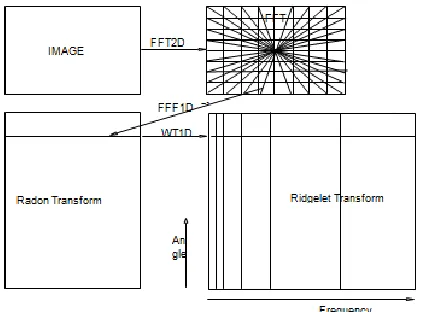
Radon transform is a superior example of Trace transform, it is integral transform containing of the integral of a function or object over straight lines, are able to convert two dimensional images and data with lines into a domain of possible line parameters [1], where each line in the image and data will give a ultimate positioned at the resultant line parameters. Fig. 1.1 shows the representation of Radon transform [2]. For the

generation of curvelet transform [3, 4], ridgelet transform and wavelet transform analysis used in the radon domain.

Fig. 1.1Radon Transform Projection.

The Radon transform of a function or object is defined by the group of line integrals in range ( , t)



[0, 2 ) R



 given by

Where



is denoted the Dirac distribution. For the ridgelet coefficients Rf(a, b, )



of an object ‘f’ are known by study of the Radon transform through

Equation (1.2) shows that the ridgelet transform analysis is related with one-dimensional (1-D) wavelet transform to the wedges of the Radon transform [5].

(i) FINITE RADON TRANSFORM

Finite Radon Transform (FRAT) analysis is based on the image pixels over a specified set of “lines” [6, 7]. Euclidean geometry analysis of Radon transform also based on finite geometry in a related modes, for finite field Zn = {0, 1... n − 1}, where ‘n’ is a prime number and

Zn is a finite field with modulo ‘n’ operations [7, 8]. For

analysis, we signify Zn∗= {0, 1... n}. Finite Radon analysis of a real function ‘f’ on the finite grid Zn2 is defined as

Where Lk, l is the set of rules that score a line on the

lattice Zn2

(2)

383 efficiency, each pixel of original image pass once for histogram analysis in Radon transform [9, 10, 11].

Ridgelet Transform

In the analysis of multi dimension, wavelets can efficiently signify only a small range of the full range of interesting behavior [12]. In consequence, wavelets are well improved for point like singularities, wherever in dimensions greater than one, stimulating singularities can be structured along lines, planes, and other non-point like structures, for which wavelets are poorly improved. A newly developed multi resolution analysis is Ridgelet analysis [13]. Its result available graphics by super sites of ridge functions or by simple elements that are in some way related to ridge functions r(a1x1+…+anxn); these are functions of n variables,

constant along hyper planes a1x1+…+anxn = c; the graph of such a function in dimension two looks like a ‘ridge’. From this we can see that we can obtain an invertible discrete ridgelet transform by taking the discrete wavelet transform (DWT) on each one FRAT plan system, (rk [0],rk[1],...,rk[p − 1]), where the path k is stable. Fig 1.3

shows implementation of ridgelet transforms [13].

Fig. 1.3Ridgelet Transform implementation

2. CURVELETTRANSFORM

Curvelet transform overcome the drawback of Wavelet Transform. Curvelet Transform is developed, Curvelet Transform is multilevel transform that not only used for a multi scale Time – Frequency analysis [14], and it is also used for the analysis of directional features. Curvelet concept is by Candes and Donoha, this transform is based on the multi resolution analysis, length and width are related anisotropic scaling law. Furthermore, edge fundamental in curvelet is defined by scaling, position and orientation parameters but in wavelets there are only scale and location parameter. Curvelet transform are used in both domain analysis frequency domain and time domain. All analysis of curvelet transform is based on the generation 1 (DCTG1) and curvelet generation 2 (DCTG2).

FIRST GENERATION CurveletsCONSTRUCTION

The first generation CurveletG1 transform [9] are based on the possibility to analyze an image with different block sizes curveletG1 analysis based on the flow graph shown in fig 1.4.

Fig.1.4 Ridgelet transform analysis for curvelet generation 1

Fig. 1.4 represent the generation of curvelet transform from ridgelet analysis [15], in this any object selected as a input and process this selected input for band pass filtering a, sub band decomposition, parameter analysis and ridgelet analysis of each square. The First Generation Discrete Curvelet Transform (DCTG1) of a continuous function f(x) creates use a sequence of scales, and a filters bank property, in this property the band pass filter ∆j is in the frequencies [22j_,22j+2_{], e.g.}

2

( )

j

,

j

f



  

2

ˆ

_{( )}

ˆ

₍₂

j

_).

j

v



v



 

Decomposition of curvelet transform are based on sub band decomposition [16], smooth portioning and ridgelet analysis, this produce that the curvelet decomposition of function in the range [22j_{, 22j}+2_].

Fig. 1.5 Decomposition of Curvelet generation 1

Before the final analysis (ridgelet analysis) of curvelet decomposition two dyadic sub band in the range 2n_and

2n+1_{, for this a isotropic wavelet transform are required,}

algorithm representation of curvelet decomposition as a superposition is in the form of any image f[i1,i2] n×n is.

1, 2 1, 2 1, 2

1

[ ] [ ] [ ]

J

j J

j

f i i Z i i w i i



 



(2.1)

Where ZJ is a coarse or flat form of the original image f and wj signifies ‘the details of f at scale 2−j_{. Thus, the}

(3)

384

1: Apply 2 dimensional wavelet transform with J scales,

2: Set Z1 = Zmin,

3: for j = 1... J do

4: Partition the sub-band with a block size Cj and apply the DRT to each block,

5: if j modulo 2 = 1 then 6: Zj+1 = 2Zj,

7: else 8: Zj+1 = Zj.

9: end if 10: end for

In this the side-length of the containing windows is doubled at every other dyadic sub-band, hence recalling the essential property of the curvelet transform at jth_for

the features of length about 2−j/2_.

3. METHODOLOGY

The execution of curvelet transform by these property are classify in two category these are curvelets via USFFT, and curvelets via Wrapping these both method are easy and transform to produce result in 2D and 3D analysis [17,18]. Both methods run in O (n2 _{logn) flops}

for n× n Cartesian arrays, with quick reversal algorithms of about the same convolution. These methods are used for large scale scientific applications analysis. Both techniques are digital transformation method and follow linear property, for the selection input these methods select input as a form of Cartesian arrays [19]. If selected image is f[t1,t2], 0 ≤ t1,t2 < n, so the analyzed output

defined as a collection of curvelet coefficients cD_{(j,l,k) is}

defined as.

1, 2

, , 1, 2 1 2 0

( , , )

[ , ],

D D

j l k t t n

C

j l k

f t t



t t











_

_

(3.1)

where each ϕDj, l, k is a digital curvelet waveform .As is standard in scientific computations, we will actually never build these digital waveforms which are implicitly defined by the algorithms; formally, they are the rows of the matrix representing the linear transformation and are also known as Rieszrepresenters. We merely introduce these waveforms because it will make the exposition clearer and because it provides a useful way to explain the relationship with the continuous-time transformation [20, 21].

Implementation of curvet coefficient

For the implementation of wavelet, Ridgelet, curvelet, matlab software 7.5 are used, For the analysis of curveletcurvelap software are used, all detail of image processing toolbox of matlab and curvelab are produce. In this implementation of algorithms by MATLAB

transform are produce To generate the curvelet coefficients of an image, select the low frequency coefficient which is stored at the center of the display. The Cartesian concentric coronae display the coefficients at altered scales, the external coronae relate to higher frequencies. There are four strips connected to respectively corona, consistent to the four key points; these are auxiliary sectioned in pointed panels. Each section signifies coefficients at an indicated scale and along the positioning suggested by the place of the panel. These are following point to generate curvelet coefficient.

1. Select image

2. forward curvelet transform, 'Take curvelet transform: fdct_wrapping'

3. generate curvelet image (a complex array)

4. display original image and the curvelet coefficient image Result analysis of two different images is produce for finest level of curvelet and wavelet transform for the variation of parameter.

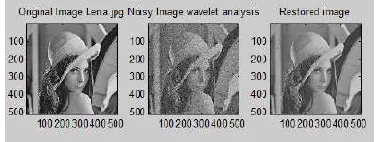
In first analysis lena.jpg image are selected for the value of N=512, standard deviation .1, no of iteration ‘0’ (in this image directly display without iteration), after this process the value of MSE and PSNR are display in the display window and resulted image are shown in fig 3.1 and fig 3.2 for curvelet transform and wavelet transform.

Fig. 3.1Lena.jpg original, noisy and restored image by wavelet transform.

Fig. 3.2 Lena.jpg original, noisy and restored image by curvelet transforms.

(4)

385 Fig 3.3 and 3.4 selected lena.jpg image are selected for the value of N=512, standard deviation 2.5, no of iteration ‘10’ (in this image directly display without iteration).

Fig. 3.3 Lena.jpg original, noisy and restored image by wavelet transform.

Fig. 3.4 Lena.jpg original, noisy and restored image by curvelet transforms.

Table 1.2 Summary of fig 3.3 & 3.4

Fig 3.5 and 3.6 selected lena.jpg image are selected for the value of N=512, standard deviation .1, no of iteration ‘5’.

Fig. 3.5 Lena.jpg original, noisy and restored image by wavelet transform

Fig. 3.6Lena.jpg original, noisy and restored image by curvelet transform

Table 1.3 Summary of fig 3.5& 3.6

Fig 3.7 and 3.8 selected lena.jpg image are selected for the value of N=512, standard deviation .5, no of iteration ‘5’.

Fig. 3.7 Lena.jpg original, noisy and restored image by wavelet transform

Fig. 3.8Lena.jpg original, noisy and restored image by curvelet transform

Table1.4 Summary of fig 3.3&3.4

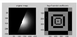
For generate curvelet coefficient this analysis produce curvelet coefficient at the centre, this analysis for lena.jpg is shown in fig. 3.9, for t1.jpg shown in fig. 3.10, for semicircle shown in fig. 3.11.

Fig. 3.9Curvelet coefficient of Lena.jpg

Fig. 3.10Curvelet coefficient of t1.jpg

(5)

386 Fig. 3.11 Curvelet coefficient of semicircle.jpg

4. Comparative Analysis of Results

This section produce the comparative analysis of wavelet and curvelet for the value of MSE and PSNR, Fig 3.11 show the comparative analysis of table no. 1.1.

Fig. 3.12Wavelt&Curvelet comparison for N= 512, standard deviation 2.5 and no of iteration 10.

Fig. 3.13Wavelt&Curvelet comparison for N= 512, standard deviation .5 and no of iteration 0.

5. CONCLUSION& FUTURE SCOPE

This paper mainly focus on the image compression and image denoising techniques of image processing, this analysis of digital image is based on wavelet transform and curvelet transform, both transform are based on the multi rate analysis and produce the recovered image at the receiver for better quality. For the analysis of image quality peak signal to noise ratio (PSNR) and mean square error (MSE) are calculate from the result analysis of both transform. To realize the efficiency of the algorithms, this tested on different types of images. The results showed that the Curvelet transform technique is practically easy and simple than the wavelet techniques. The result analysis show that the variation of standard deviation, no of iteration and value of N, by the variation of these parameter different types of result are produce for both transform, after the comparative analysis we can see that the curvelet transform are better than the wavelet transform. The fields in which future scope of curvelet transform can extended are curvelet algorithms in 3D and higher dimension, for running image, large images, other domain rather than frequency, field of medical science curvelet transform produce better result than the other transform but some field of medical science are vacant, so the future scope in this field are available.

REFERENCES

[1]. J. Ma, M. Fenn, “Combined complex ridgelet shrinkage and total variation minimization,” SIAM J. Sci. Comput., 28 (3), 984-1000 (2006).

[2]. Sigurdur Helgason, “Radon Transform,” Second Edition.

[3]. F. Matus and Jan Flusser, “Image Representation via Finite Radon Transform,” IEEE Transaction on pattern analysis and machine intelligence, Vol. 15, No. 10, 1993.

[4]. Yves Nievergelt, “Exact Reconstruction Filters To Invert Radon Transforms With Finite Elements,” Journal Of Mathematical Analysis And Applications 120, 288314 (1986).

[5]. Michael E. Orrison, “Radon Transforms And The Finite General Linear Groups,” This Article Appeared In Forum Mathematicum, No. 1, 97-107, 2004.

[6]. Lauren A. Ostridge and John C. Bancroft, “An investigation of the Radon transform to attenuate noise after Migration,” CREWES Research Report, Vol. 19, 2007.

[7]. M. Hasan, AL.Jouhar and Majid A. Alwan, “Face Recognition Using Improved FFT Based Radon by PSO and PCA Techniques,” International Journal of Image Processing (IJIP), Vol. 6, 2012.

(6)

387 edge-preserving image reconstruction,” Signal Process., 82 (11), 1519-1543 (2002).

[9]. Alexander Kadyrov and Maria Petroa, “The Trace Transform and its application,” IEEE Trans.Pattern Analysis and Machine Intelligence, Vol.23, No.8, 2001. [10].Y. Lu and M. N. Do, “Multidimensional directional filter

banks and surfacelets,” IEEE Trans. Image Process., vol. 16, no. 4, pp. 918–931, 2007.

[11].Minh N. Do, Martin Vetterli, “The Finite Ridgelet Transform for Image Representation,” IEEE TRANSACTIONS ON IMAGE PROCESSING.

[12].H. Douma and M. de Hoop, "Leading-Order Seismic Imaging Using Curvelets," Geophysics, vol. 72, no. 6, pp. S231–S248, 2007.

[13].S. Foucher, V. Gouaillier and L. Gagnon, “Global Semantic Classification of Scenes using Ridgelet Transform,” R&D Department, Computer Research Institute of Montreal, 2004.

[14].M.J. Fadili, J.-L. Starck, “Curvelets and Ridgelets,” October 24, 2007.

[15].E. Candès and L. Demanet, “The curvelet representation of wave propagators is optimally sparse,” Commun. Pure Appl. Math. pp. 1472–1528, 2005, vol. 58, no. 11.

[16].B. S. Manjunath et al, “Color and Texture Descriptors,” IEEE Transactions CSVT, 703-715, 2001, 11(6).

[17].E. Candes, D. Donoho, “New tight frames of curvelets and optimal representations of objects with piecewise singularities,” Comm. Pure Appl. Math., 57, 219-266 (2004).

[18].Jianwei Ma and Gerlind Plonka, “The Curvelet Transform,” IEEE SIGNAL PROCESSING MAGAZINE, 118-133, 2010.

[19].J. Starck, "Gray and Color Image Contrast Enhancement by the Curvelet Transform," IEEE Trans. Image Processing, vol. 12, no. 6, pp. 706–717, 2003.

[20].R. Neelamani et al., "Coherent and Random Noise Attenuation Using the Curvelet Transform," The Leading Edge, vol. 27, no. 2,2008, pp. 240–248.