PURE Insights
Volume 3
Article 9
2014
Predicting the Cy Young Award Winner
Stephen Ockerman
Western Oregon University, [email protected]
Matthew Nabity
Western Oregon University, [email protected]
Follow this and additional works at:
https://digitalcommons.wou.edu/pure
Part of the
Numerical Analysis and Computation Commons
This Article is brought to you for free and open access by the Student Scholarship at Digital Commons@WOU. It has been accepted for inclusion in PURE Insights by an authorized editor of Digital Commons@WOU. For more information, please [email protected].
Recommended Citation
Predicting the Cy Young Award Winner
Abstract
Here we examine the application of a decision model to predicting the winner of the Cy Young Award. We investigate a current model cast as a linear programming problem and explore its ability to correctly predict award winners for recent seasons of professional baseball. We suggest the addition of another baseball statistic which leads to a new model. We explore the success of both models with numerical experiments and discuss the results.
Keywords
linear programming, mathematical model, sabermetrics
Predicting the Cy Young Award Winner
Stephen Ockerman and Matthew Nabity
1. Introduction
The game of baseball has long been associ-ated with collecting and analyzing empirical data. Since the creation of Major League Baseball in 1903, various numerical measurements have been recorded and invented.
These records have been used by fans of the game to assess teams and players, and more re-cently, by those interested in further studying the game. The mathematical study of baseball statis-tics is often referred to as sabermetrics, named after the Society for American Baseball Research (SABR) [3]. The practice of sabermetrics is de-picted in the book Moneyball and in the recent movie adaptation. Mathematical analysis of the many facets of the game of baseball has been grow-ing steadily in recent years.
In 2005, a mathematical model to predict the winner of MLB’s Cy Young Award was suggested by Sparks and Abrahamson [5]. This model used a di↵erent approach than the methodologies com-mon to sabermetrics. The authors attempted to use on-field statistics to forecast o↵-field assess-ments. The Cy Young Award is awarded to the most outstanding pitcher in each of the American and National Leagues, and the winners are chosen by voting members of the Baseball Writers Asso-ciation of America. The mathematical model was formulated not to predict who should be awarded the Cy Young Award but to accurately predict how the award voting would go. That is, the model hoped to use the current season of statistics to pre-dict how voters would rank the pitchers.
Data from the 1993 season through the 2002 season was used, specifically five common statis-tics: wins, losses, earned run average, team
win-ning percentage, and strikeouts. Weights for a weighted average were determined by formulating and solving a linear programming problem. A lin-ear programming problem has a linlin-ear function of the unknowns. The objective is to maximize or minimize this function subject to constraints that are also linear. In this model, weights for each of the statistics were determined and then used to compute a numerical score for each player. The player with the highest score was expected to win the award, the player with the second highest score would finish in second place, and the player with the next highest score would finish in third place. The model using all 20 seasons of data did not have a solution. After a closer inspection of the data, the authors removed the statistics from the American League (AL) in 1995. With this single constraint removed, the model correctly predicted the voters’ choice for the top three finishers in each league in every year except for the AL in 1995. In this isolated case, the winner was correctly identi-fied, but second and third places were not.
Nearly a decade later, this work began with a central question, does this model accurately cap-ture the attitude of the voters today? Those that follow the game of baseball may be aware of the numerous statistics available and the often in-tense debates about which ones matter more for in-season performance and post season accolades. Many baseball fans may also be aware of recent emphasis on statistics such as WHIP, walks and hits per inning pitched, or WAR, wins above re-placement.
To explore the relevance of the model, we revisit the formulation of Sparks and Abraham-son’s model and apply it to more recent seasons, namely the 2005 through 2013 seasons. Based on
A publication of the Program for Undergraduate Research Experiences at Western Oregon University
!
digitalcommons.wou.edu/pure ©2014
the numerical results, we explore the addition of another statistic and suggest an updated version of the model. We report numerical results of our new model and discuss the results of our modeling e↵orts.
2. The Mathematical Model
When examining an award for pitchers, we need to understand the position. There are two major types of pitchers. The first, the starting pitcher, typically begins the game and pitches un-til relieved. The second, the relief pitcher, is any player that is not in the starting rotation. In re-cent years, the work of relief pitchers, specifically those that finish the game, has been increasingly appreciated by Cy Young voters. In fact, the Na-tional League (NL) Cy Young winner in 2003, ´Eric Gagn´e, was such a relief pitcher, often called a closer. Closers are usually judged by di↵erent stan-dards than starting pitchers.
The model developed by Sparks and Abra-hamson does not apply to the 2003 season in the NL as they restricted their analysis to include only starting pitchers. For the 2005 season, the model correctly predicted Chris Carpenter for the NL winner. In the AL that year, the consensus was that there was no stand out performance and many believed Mariano Rivera, a relief pitcher, would win. The mathematical model correctly predicted Bartolo Col´on would be the AL winner, but Mari-ano Rivera, who finished second in the voting, was not included in the analysis as he was not a start-ing pitcher.
Other attempts to predict the Cy Young Award winner have been made using di↵erent mathematical techniques, for example the data mining approach by Smith et al [4]. Using a Bayesian classifier, the authors examined data from the years 1967 to 2006 and were more than 80% correct when restricting their analysis to only starting pitchers [4]. Accuracy su↵ered when in-cluding relief pitchers. Due to the difficult na-ture of including relief pitchers, the most successful models currently consider only starting pitchers.
The statistics used in the original model
in-clude wins (W), losses (L), earned run average (ERA), strikeouts (K) and team winning percent-age (TWP). The first four of these measurements are fairly common, but TWP is not necessarily a direct assessment of an individual. One of the modeling assumptions is that players on better teams get more exposure and potentially more credit for the success of the team. To make the data easier to compare, Sparks and Abrahamson put all five statistics on the same scale, zero to ten, using simple linear transformations. The parame-ters were chosen so that a score near ten reflects a historic performance and a score near zero re-flects a performance of little interest to voters. For pitcheriin year j, they defined the following:
pij1 = W
3 (2.1)
pij2 =10
✓
15 L 15
◆
(2.2)
pij3 =12.5 2.5(ERA) (2.3) pij4 =20(T W P 0.25) (2.4)
pij5 =10
✓
K 50
333
◆
. (2.5)
Using the scaled data, a score for pitcheriin year j, Sij, can be compute as weighted sum of these parameters:
Sij = 5
X
k=1
xkpijk,
where the xk are to be determined so that the pitcher that wins has the highest score in the league for yearj, the second-place finisher should have the second highest score, and the third-place finisher should have the third highest score.
Sparks and Abrahamson required that the nonnegative weights add up to one so that each scoreSij was a convex combination of the param-eters pijk, k = 1,2, . . . ,5. The formulation thus far is to find numbersx1 through x5 so that all of
the following are true:
5
X
k=1
xk= 1 (2.6)
where m is the number of seasons used. The straints 2.7 and 2.8 are close to the types of con-straints that appear in a linear programming prob-lem. A linear programming problem is character-ized by linear functions of the unknowns and linear inequalities and equalities of the constraints [2]. The goal is to maximize or minimize a specific ob-jective subject to certain constraints. For example, if p1 and p2 are two measures of performance
de-scribed above, and the goal is to find weights w1
andw2 that would maximize the weighted average w1p1 +w2p2, then the overall problem could be
expressed as
Maximize: w1p1+w2p2
Subject to: p1+p2b p1 0, p2 0,
wherebis some number derived from the context. A successful solution to this simple linear program would compute values for w1 and w2. For details
on linear programming problems and related algo-rithms, see [2]. Examining 2.8 more closely, we see that for each year j
5
X
k=1
xkp1jk > 5
X
k=1
xkp2jk > 5
X
k=1
xkp3jk,
or rearranging terms we have constraints of the form
5
X
k=1
xk(p1jk p2jk)>0, j = 1,2, . . . , m,
5
X
k=1
xk(p2jk p3jk)>0, j = 1,2, . . . , m. (2.9)
The authors made these inequalities not strict by replacing zero with a small positive number. This adjustment made it so that constraints 2.7 and 2.9 specify the feasible region for a linear programming problem. Mathematically speaking, all that was needed now was something to optimize, that is, an objective function.
Sparks and Abrahamson set up a linear pro-gramming problem in which the score S1j for all years j in the data set was maximized. To accom-plish this, they chose to maximize the sum of all
winners over the years in the data set. In linear programming terms, this was selected as the objec-tive function for the maximization problem. The final form of the problem was as follows:
Problem (LP1-CY)
Givena >0, findx= (x1, . . . , x5) that satisfies:
Maximize: F(x) = m
X
j=1
S1j (2.10)
= m X j=1 5 X k=1 xkp1jk
subject to:
5
X
k=1
xk(p1jk p2jk) a, j= 1, . . . , m (2.11)
5
X
k=1
xk(p2jk p3jk) a, j= 1, . . . , m (2.12)
5
X
k=1
xk = 1 (2.13)
xk 0, k= 1, . . . ,5. (2.14)
We note that when using data from all 20 sea-sons, no feasible solution was found to exist. The 1995 season caused problems for the model LP1-CY and the authors chose to delete the AL in-formation from that year. Removing this single constraint allowed the linear programming pack-age from Mathematica to compute the following weights:
x1= 0.578084, (W) x2= 0.00999357, (L) x3= 0.197600, (ERA) x4= 0.0784757, (TWP) x5= 0.136747, (K).
2.1. Numerical Results Part One
To explore the relevance of this model on more recent seasons, we performed a few numerical ex-periments. All computations were done using the linear programming capabilities of standard func-tions inMatlabR 2013a. First, we used the orig-inal model formulation but only constraints from the past nine seasons, 2005 to 2013. As in the initial attempt by the original authors, no feasible solutions were found. Recall that the original au-thors had to remove a constraint, namely the 1995 season data from the AL. This may have been easy to identify as there was a players strike that ended the 1994 season and carried on into the 1995 sea-son. When looking at more recent seasons, we had no obvious seasons to look at.
To gain some insight into the most recent nine seasons of data, we computed the scores for the top three finishers using the original weights computed by Sparks and Abrahamson for the data from 1993 through 2002. We found that the overall winner in the AL was correctly identified in six of the nine years: 2005, 2006, 2008, 2011, 2012, and 2013. Of these, the model did not properly account for re-lief pitcher Mariano Rivera in 2005, and had the second place and third place finishers in the wrong order in 2012. The story was about the same for the results in the NL. The model correctly identi-fied the top three finishers in five of the nine years: 2005, 2006, 2007, 2010, and 2011.
Collectively, the weights determined by the LP1-CY were only successful in predicting the win-ners in both leagues in 2006 and 2011. We were un-able to identify a pattern for the success or failure of the model, and there were no obvious seasons to consider removing from the set of constraints. Based on the assumption that the voters’ attitudes have been changing in recent years, we set out to incorporate additional information.
3. A New Model
Though there have been successful relief pitch-ers lately, we also opt to restrict our analysis to starting pitchers. Despite the fact that the weights
computed by the original authors suggest that the number of losses seems unimportant to voters, we base our model on the five original statistics and choose to include an additional statistic. Walks plus hits per inning pitched (WHIP) is a saber-metric measurement that has been used to assess pitchers for over three decades. In recent years this statistic has found its way into MLB box scores on popular sports websites. The measure-ment attempts to measure a pitcher’s e↵ectiveness against batters. The lowest single-season WHIP in MLB history, 0.7373, was recorded by Pedro Mar-tinez during the 2000 season while playing for the Boston Red Sox [1]. Using this value as a historic performance, we define the transformation
pij6=10 (2 W HIP) 2.627, (3.1)
to incorporate WHIP into the model based on LP1-CY. Here a WHIP of 0.7373 would score ten points. Adding this component to the data and us-ing the scaled data from LP1-CY, we now consider the weighted sum or objective function
Sij = 6
X
k=1
xkpijk,
follow-ing:
Problem (LP2-CY)
Givena >0, findx= (x1, . . . , x6) that satisfies:
Maximize: F(x) = m
X
j=1
S1j (3.2)
= m
X
j=1 6
X
k=1 xkp1jk
subject to:
6
X
k=1
xk(p1jk p2jk) a, j= 1, . . . , m (3.3)
6
X
k=1
xk(p2jk p3jk) a, j= 1, . . . , m (3.4)
6
X
k=1
xk = 1 (3.5)
xk 0, k= 1, . . . ,6. (3.6)
The incorporation of an additional measurement changes both the objective function and the con-straints that define the feasible region. We now seek six weights to help capture the voters’ atti-tude.
3.1. Numerical Results Part Two
In this section we report the results of fur-ther numerical experiments using both the original model LP1-CY and our updated version LP2-CY. Here we examine solutions to each of the models for various sets of constraints. The goal is to iden-tify weights that most accurately predict the top three finishers.
We began with data from both leagues for the most recent seasons, 2005 through 2013. Recall from the previous numerical experiments, there was no feasible solution to LP1-CY using data from these nine seasons. We observed the same for our new model LP2-CY using these same con-straints. To investigate this further, we turned to the original weights computed using the 1993 through 2002 seasons, excluding the AL results from 1995. Looking at the NL results using these
weights, we noticed that there seemed to be a change after the 2007 season. This motivated us to restrict our constraints to data from the most recent six seasons.
Experiment 1
Here we used data from the past 6 seasons, 2008 through 2013, for both leagues. For LP1-CY, we computed the weights to be
x1 = 0.000000, (W) x2 = 0.051184, (L) x3 = 0.780348, (ERA) x4 = 0.083859, (TWP) x5 = 0.084608, (K),
and for LP2-CY we found the weights to be
x1 = 0.000000, (W) x2 = 0.051184, (L) x3 = 0.780348, (ERA) x4 = 0.083859, (TWP) x5 = 0.084608, (K) x6 = 0.000000, (WHIP).
We found the weights to be the same for either model as the weight for WHIP was determined to bex6 = 0. Restricting our analysis to the seasons
2008 through 2013 seems to indicate that our new statistic may be extraneous. Here wins and WHIP do not seem to be factors, and ERA is the main component emphasized.
1st 2nd 3rd
’08 C. Lee R. Halladay F. Rodr´ıguez
5.9328 5.3351 5.3341
’09 Z. Greinke F. Hernandez J. Verlander
6.5204 6.1234 4.2513
’10 F. Hernandez D. Price C. Sabathia
6.1037 5.6810 4.7606
’11 J. Verlander J. Weaver J. Shields
6.4852 6.1389 5.3232
’12 D. Price J. Verlander J. Weaver
6.0084 5.8145 5.3489
’13 M. Scherzer Y. Darvish H. Iwakuma
5.5325 5.5315 5.5305
Table 3.1: AL Top Cy Young finishers and associ-ated scores using weights from experiment 1
1st 2nd 3rd
’08 T. Lincecum B. Webb J. Santana
5.8559 4.3567 5.9895
’09 T. Lincecum C. Carpenter A. Wainwright
6.2167 6.5219 5.7973 ’10 R. Halladay A. Wainwright U. Jim´enez
6.1796 6.0552 5.2308
’11 C. Kershaw R. Halladay C. Lee
6.5851 6.5462 6.4261
’12 R. Dickey C. Kershaw G. Gonz´alez
5.5401 5.9495 5.3495 ’13 C. Kershaw A. Wainwright J. Fernandez
7.3848 5.2383 6.3602
Table 3.2: NL Top Cy Young Finishers and Asso-ciated Scores, experiment 1
identified half the time and all top three finish-ers were correctly identified in only two of the six years. While we were able to compute a solution to both LP-CY1 and LP-CY2, the weights are not performing well and we opt to further explore the constraints.
Experiment 2
We now restrict the constraints to data from the 2009 through 2013 seasons for both leagues. That is, we removed the statistics from the 2008 season. Using only the most recent five seasons, LP1-CY produced the same weights as in the first experiment. The scores for the top three finishers are they same as those reported in Table 3.1 and
Table 3.2. We saw that these weights correctly identified all top three finishers in the AL but were much less successful in the NL, especially for the two most recent seasons as illustrated in Table 3.2. Using LP2-CY with the constraints from the 2009 through 2013 seasons, we found the weights to be
x1 = 0.301385, (W) x2 = 0.048033, (L) x3 = 0.000000, (ERA) x4 = 0.000000, (TWP) x5 = 0.197455, (K) x6 = 0.453127, (WHIP).
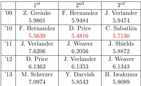
Now WHIP and wins are more important compo-nents, whereas both ERA and TWP are nonfac-tors. Using these weights, we compute the scores for the top three finishers in each league and com-pare the performance to the results in the first ex-periment. Table 3.3 shows the results for the AL using the weights computed by LP2-CY for the second experiment. Again, incorrect predictions are highlighted in red.
1st 2nd 3rd
’09 Z. Greinke F. Hernandez J. Verlander
5.9801 5.9484 5.9474
’10 F. Hernandez D. Price C. Sabathia
5.5639 5.4816 5.7130
’11 J. Verlander J. Weaver J. Shields
7.6206 6.2056 5.8872
’12 D. Price J. Verlander J. Weaver
6.1363 6.1353 6.1343
’13 M. Scherzer Y. Darvish H. Iwakuma
7.0974 5.8543 5.8089
Table 3.3: AL Top Cy Young Finishers and Asso-ciated Scores, experiment 2
season. If these scores are compared to the scores calculated in Table 3.3, we see that Max Scherzer had a higher score in Table 3.3. This suggests that the addition of WHIP may have been helpful for seasons such as this when players have comparable statistics.
Unfortunately, the weights computed by LP2-CY failed to correctly identify any of the fin-ishers for the 2010 season. We will investigate this further in ensuing experiments. To fully assess the performance of our model we turn our attention to the NL results. Table 3.4 shows the scores for the top three NL finishers when using weights com-puted by LP2-CY and only data from the 2009 through 2013 season. Here we see a much di↵erent story than for the AL results.
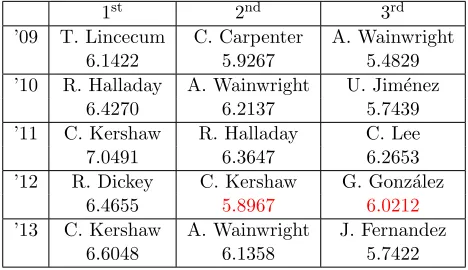
We can look at Table 3.2 for the performance of LP1-CY in the second experiment as the com-puted weights remained the same. These weights correctly predicted the winner in only three of the five years, 2010, 2011, and 2013, and correctly identified all three finishers only in 2010 and 2011. For comparison, the weights computed by LP2-CY accurately captured all first place finishers over the years in question. The only incorrect score oc-curred in 2012 where second and third place were out of order. This is a significant improvement
1st 2nd 3rd
’09 T. Lincecum C. Carpenter A. Wainwright
6.1422 5.9267 5.4829
’10 R. Halladay A. Wainwright U. Jim´enez
6.4270 6.2137 5.7439
’11 C. Kershaw R. Halladay C. Lee
7.0491 6.3647 6.2653
’12 R. Dickey C. Kershaw G. Gonz´alez
6.4655 5.8967 6.0212
’13 C. Kershaw A. Wainwright J. Fernandez
6.6048 6.1358 5.7422
Table 3.4: NL Top Cy Young Finishers and Asso-ciated Scores, experiment 2
from the results in Table 3.2 and may o↵set the issue with the 2010 season in the AL. When exam-ining the results from both leagues, it seems that for the seasons under consideration, LP2-CY more accurately predicts not only the winner but also
the top three finishers.
Additional Experiments
We performed several other experiments to at-tempt to identify problematic seasons. We found no feasible solutions to both LP1-CY and LP2-CY for the following sets of constraints: all data from 2005 through 2013, all data from 2005 through 2013 when omitting 2010 AL statistics, all data from 2005 through 2013 omitting all 2010 data, all data from 2005 to 2013 omitting 2010 AL statistics and 2012 NL statistics, all data from seasons 2005 through 2008, and all data from 2009 through 2013 omitting 2010 AL statistics.
We found two sets of constraints that gener-ated two di↵erent sets of weights for LP2-CY when there was no feasible solution to LP1-CY. These configurations included the 2009 through 2013 sea-sons when omitting the 2010 AL data and the 2012 NL data and the 2009 through 2013 seasons when omitting the 2012 NL data. In either case, the weights switched the second place and third place finishers in the NL in 2012 as we saw in the sec-ond experiment in Table 3.4. The success of these other weights in the AL was not as good as what we observed in the second experiment in Table 3.3.
4. Discussion of Results
WHIP, we plan to further investigate refinements to LP2-CY. A closer examination of individual seasons in both leagues may shed some light on problematic constraints or seasons. Additionally, the incorporation of additional sabermetric mea-surements may help better capture the voters’ be-havior. We plan to investigate possible model im-provements in time for the coming postseason.
References
[1] Sports Reference LLC. Baseball-reference.
http://www.baseball-reference.com,
De-cember 2013.
[2] David Luenberger and Yinyu Ye. Linear and Nonlinear Programming. Springer, 3rd edition, 2008.
[3] SABR. Society for american baseball research. http://sabr.org, December 2013.
[4] Lloyd Smith, Bret Lipscomb, and Adam Simkins. Data mining in sports: Predicting the cy young award winners. J. Comput. Sci. Coll., 22(4):115–121, 2007.