R E S E A R C H
Open Access
Boundary value problems for periodic
analytic functions
Pei Dang
1, Jinyuan Du
2,3*and Tao Qian
4*Correspondence:
2School of Science, Linyi University,
Linyi, Shandong 276000, P.R. China
3Department of Mathematics,
Wuhan University, Wuhan, 430072, P.R. China
Full list of author information is available at the end of the article
Abstract
In this paper boundary value problems for periodic analytic functions are discussed. We first introduce definitions of principal part and order at±∞ifor periodic analytic functions through detailed analysis. Then Riemann boundary value problems for
periodic analytic functions with finite order at±∞iare formulated. Based on those,
by using the exponential conformal mapping, Riemann boundary value problems for periodic sectionally holomorphic functions with periodic closed and periodic quasi-closed contours as their jump curves are solved. The method that we use here has computational advantages compared with the tangent mapping one used in solving the classical problems. Several types of Hilbert boundary value problems on the real axis and the circumferences for periodic analytic functions are also solved.
MSC: 30E25; 45E05
Keywords: principal part; order at±∞i; periodic Riemann boundary value problem; periodic Hilbert boundary value problem
1 Introduction
The theory of boundary value problems for analytic functions is an important branch of complex analysis. It has ample applications due to the fact that many practical problems in mechanics, physics, and engineering may be converted to boundary value problems or sin-gular integral equations [–]. Boundary value problems for analytic functions have been systematically investigated in the related literature (see, for instance, [–]). In the mono-graph [] Lu first introduced the so-called periodic Riemann boundary value problems (PR problems) and periodic Hilbert boundary value problems (PH problems) motivated from the periodic problems in plane elasticity. More general formulations of such prob-lems are for automorphic functions which were first studied by Gakhov and Chibrikova [, ]. From the practical point of view, the periodic boundary value problems are consid-erably important. In particular, by using the solutions and methods for PR problems and PH problems one can effectively solve a number of periodic problems in plane elasticity [–].
In [], Lu mainly discussed PR problems with periodic closed contour as the jump curve and PH problems on the real axis for bounded solutions. He transferred periodic boundary value problems to standard Riemann boundary problems and Hilbert boundary problems by the tangent conformal mapping. The theme of unbounded solutions at the infinity has not been well addressed, although some results were predicted []. The predicted results,
however, are not accurate, for there is no detailed and rigorous analysis for the behavior of the solutions at the infinity.
In the present paper, we will discuss in depth three different types of problems: (i) the Riemann boundary value problem for periodic sectionally holomorphic functions with periodic closed contour or quasi-closed contour as jump curves; (ii) the Hilbert bound-ary value problem on the real axis for the periodic holomorphic function in the upper half-plane; and (iii) the Hilbert boundary value problem on periodic circumferences for periodic holomorphic functions in the disks, being the interior regions of a set of peri-odic circumferences. In the next section, we shall introduce definitions of the principal part and order at the infinity for periodic holomorphic functions by using the exponential conformal mapping. Then Riemann boundary value problems for periodic holomorphic functions with finite orders at±∞iare presented in Section . We transfer the PR prob-lem to a standard Riemann boundary value probprob-lem by the exponential conformal map-ping, and the solution formula and a set of conditions for the solvability are obtained. In Section , the periodic Hilbert boundary value problem on the real axis and on periodic circumferences are discussed, respectively, in two ways. The first is the so-called reflex extension and the second is the so-called regular factor method.
Periodic Riemann boundary value problems and periodic Hilbert boundary value prob-lems have applications to global asymptotic analysis for orthogonal polynomials on the real axis. To keep the present paper within a reasonable bound the application aspect will be postponed to a forthcoming paper.
2 Order of periodic analytic functions at the infinity
Assume
L=
+∞
k=–∞
Lk (.)
is a set of smooth closed contours, non-intersecting to each other, with the same shape and size, arranged horizontally with periodaπ (a> ) and oriented counter-clockwise (see Figure ), which is called a periodic closed contour. The interior region ofLkis denoted by
S+k and the exterior ofLbyS–. We may assumeO∈S+and±aπ/∈S–, which is always possible through a translation of the axes if necessary.
A set S is called the periodic set with the periodaπ (a> ), if z±aπ∈S for any
z∈S. So,S–,S+, andLare all periodic sets with the periodaπ, where
S+=
+∞
k=–∞
S+k. (.)
The PR problem is formulated as follows (see []): Find a periodic sectionally holomor-phic function(z) withLas the jump curve such that
+(t) =G(t)–(t) +g(t), t∈L, (.)
whereGandgare given onLwith the periodaπ, that is,
G(t+aπ) =G(t), g(t+aπ) =g(t), (.)
satisfying the normal type condition
G(t)= , t∈L, (.)
and the Hölder conditions
G∈H(L), g∈H(L). (.)
In general, infinity∞should not be an isolated singular point of the solution of the PR problem (if any). In relation to this, its principal part and order at infinity∞are not well defined in the classical sense. LetC be the complex plane, and, forz∈C, x=Rez, and
y=Imz. For anyh∈R, we call the sets
N(+∞i,h) ={z:y=Imz>h}, N(–∞i,h) ={z:y=Imz<h} (.)
neighborhoods of +∞iand –∞i, respectively. The exponential conformal mapping
w=eaiz, z∈C, (.)
maps, respectively, the upper strip region and the lower strip region
Nh+=
z:Imz>h, –
aπ≤Rez≤ aπ
,
Nh–=
z:Imz<h, –
aπ≤Rez≤ aπ
(.)
into the interior and exterior of the circle{w:|w|=e–h/a}, maps the infinity accumulation
pointz= +∞iofNh+ and the infinity accumulation point z= –∞iofN–
h tow= and
Let+(z) be a holomorphic function with the periodaπon the neighborhood of +∞i,
denoted by+∈A+aπ. Then
+∗(w) =+(z) =+
–ai lnw
, <|w|<e–ah, (.)
is well defined and analytic by the Painlevé theorem, where the logarithm functionlnwis the principal branch in the complex plane cutting along (–∞, ],i.e.,
lnw=ln|w|+iarg(w) –π≤arg(w) <π ,w= , (.)
which is the inverse mapping of the restriction of the exponential mapping (.) on the strip regionS={z:Imz> , –π≤Rez<π}. Thus,+∗ has a Laurent expansion, then we
know easily that there is also the unique expansion in the series form for+[, ], that
is,
+(z) =
+∞
–∞ aje
ijz
a (Imz>h), (.)
where
aj=
π
ϒ
+(z)e–ijza dz,
ϒ:=
z:z=x+ir, –aπ
≤x≤
aπ
,ris an arbitrary constant greater thanh
(.)
orϒ:=
z:z=x+ih, –aπ
≤x≤
aπ
, while+is continuous to it.
If the expansion in (.) is
+(z) =
+∞
j=m
a–je–
ijz
a witha
–m= ,z∈Nh+, (.)
then we say that+has the pole of ordermatz= +∞i, or simply, orderm, denoted as
eOrd[+](+∞i) =m, which is just equivalent to that its associated function+∗ has the
pole of ordermatw= denoted asOrd[+
∗]() =m. We agree that the pole of ordermis just the zero point of order –m. Thus, we has
eOrd+(+∞i) =m ⇐⇒ Ord+∗() =m. (.)
If–(z) is a holomorphic function with the periodaπ on the neighborhood of –∞i,
denoted by–∈A–aπ, similarly, it also has the unique expansion in the series form
–(z) =
+∞
–∞
bje
ijz
where
bj=
π
ϒ
–(z)e–ijza dz,
ϒ:=
z:z=x+ir, –aπ
≤x≤
aπ
,ris an arbitrary constant smaller thanh
orϒ:=
z:z=x+ih, –aπ
≤x≤
aπ
, while–is continuous to it.
(.)
In particular, if
–(z) =
+∞
j=m
bje
ijz
a withb
m= ,z∈Nh–, (.)
we say that–has the pole of ordermatz= –∞i, denoted aseOrd[–](–∞i) =m, which is just equivalent to that its associated function
–∗(w) =–(z) =–
–ai lnw
, |w|>e–ah, (.)
where the mapping (.) has the pole of ordermatw=∞, denoted asOrd[–∗](∞) =m,
i.e.,
eOrd–(–∞i) =m ⇐⇒ Ord–∗(∞) =m. (.)
3 Periodic Riemann boundary value problems
In the section, we give the formulation and transformation of periodic Riemann boundary value problems. Then both the expression of the solution and the condition of solvability are obtained in closed form.
3.1 Formulation of the problem
In PR problem (.), ifis required to have at most order n at +∞iand ordermat most at –∞i, then the problem is denoted byPRm,n.
PRm,nproblem: Find a periodic sectionally holomorphic function(z) withLas the jump
curve such that
⎧ ⎪ ⎨ ⎪ ⎩
+(t) =G(t)–(t) +g(t), t∈L, eOrd[](+∞i)≤n,
eOrd[](–∞i)≤m,
(.)
whereGandgare defined onLsatisfying (.), (.), and (.).Lis the periodic closed contour given in the last section. In addition,Lcan also be the periodic quasi-closed con-tour given below.
A set of smooth open arcsLj=ajaj+(j= ,±,±, . . .) is called a periodic quasi-closed
contours, if theLjhave the same shape and size, arranged horizontally with periodaπ
(a> ),aj= (j–)aπand the tangents ofLjat their ends are parallel. For concreteness,
Figure 2 A periodic quasi-closed contour.
(see Figure ). The particular caseLj= [(j–)aπ, (j+)aπ] is worth paying attention to,
for in that caseLreduces to the real axis.
3.2 Transformation of the problem
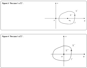
LetLbe a periodic closed contour or a periodic quasi-closed contour. The following dis-cussions and even all the results for the two cases are essentially the same. For example, under the mapping (.), the image ofLon thew-plane, denoted by, is a smooth closed
contour surroundingw.divides thew-plane into the interior region+and the
exte-rior region–(see Figure and Figure ), which are, respectively, the images of the strip regions
S+=
z:z∈S+, –
aπ≤Re(z)≤ aπ
,
S–=
z:z∈S–, –
aπ≤Re(z)≤ aπ
.
(.)
In the sequel, for simplicity, we will take
w=
, when ∈+(Figure ),
, when /∈+(Figure ). (.)
Remark . WhenLis a periodic quasi-closed contour, it is possible that /∈+. For
example,Lcan be the real axis. Of course, we may always take ∈+ by a translation transform.
As before, we easily see that, if(z) is a periodic sectionally holomorphic function with
Lbeing the jump curve, then, under the mapping (.) or (.), its associated function,
∗(w) =
–ai lnw
, w∈C\, (.)
is a sectionally holomorphic function, whereis the jump curve and
±∗(τ) =±(t) withτ=eait ∈(t∈L). (.)
Figure 3 The case 1∈+.
Figure 4 The case 1 /∈+.
R∗m,nproblem: Find a sectionally meromorphic function∗(w) having possible pole point atw= , withas the jump curve, such that
⎧ ⎪ ⎨ ⎪ ⎩
+∗(τ) =G∗(τ)∗–(τ) +g∗(τ), τ∈,
Ord[∗]()≤n,
Ord[∗](∞)≤m,
(.)
where
G∗(τ) =G
–ai lnτ
, g∗(τ) =g
–ai lnτ
, τ∈, (.)
with the mapping (.). Obviously,
G∗(τ)= , τ ∈. (.)
It is easy to prove that
G∗∈H(), g∗∈H(). (.)
Conversely, if∗is the solution ofR∗m,nproblem (.), then
(z) =∗eaiz , z∈C\L, (.)
is the solution ofPRm,nproblem (.). In fact, it is obvious that the aboveis a periodic
We summarize the above discussion as follows.
Lemma . Under the relationship(.)or(.),PRm,nproblem(.)is equivalent to R∗m,n
problem(.).
Let
(w) =wn∗(w), w∈C\, (.)
G(τ) =G∗(τ) and g(τ) =τng∗(τ), τ∈. (.)
Then we transfer theR∗m,nproblem to the following Riemann boundary value problem.
Rm+nproblem: Find a sectionally holomorphic function(w), withas the jump curve,
such that
+(τ) =G(τ)–(τ) +g(τ), τ ∈,
Ord[](∞)≤m+n. (.)
This is a classical Riemann boundary value problem [, ].
Lemma . Under the relationships(.)and(.),R∗m,nproblem(.)is equivalent to Rm+nproblem(.).More specifically,if∗is the solution of R∗m,nproblem(.),thenis
the solution of Rm+nproblem(.).Conversely,ifis the solution of Rm+nproblem(.),
then∗is the solution of R∗m,nproblem(.).
3.3 Solution of problem We call
κ=IndLG(t) =
π
argG(t)L
(.)
the index ofGor the index ofPRm,nproblem (.). Obviously, it is just the index ofG∗=G
orR∗m,nproblem (.) andRm+nproblem (.),i.e.,
κ=IndG∗(τ) =
π
argG∗(τ)≡ π
argG(τ)
=IndG(τ). (.)
Rm+nproblem (.) is an ordinary Riemann boundary value problem. From [, ], we
know that, whenm+n+κ≥–, the general solution ofRm+nproblem (.) is
(w) =X(w)
(w) +Pm+n+κ(w)
, w∈C\, (.)
wherePris an arbitrary polynomial of degree not greater thanr(Pr≡ ifr< ), denoted
asPr∈r. The canonical function
X(w) = ⎧ ⎨ ⎩
e(w), w∈+,
(w–w)–κe(w), w∈–,
wherewis given by (.),
(w) = πi
log[(τ–w)–κG(τ)] τ–w dτ–C
=
πi
log[(τ–w)–κG∗(τ)]
τ–w dτ–C, (.)
with an arbitrary complex constantCand an arbitrary branch of the logarithm, and
(w) = πi
g(τ)
X+
(τ)(τ–w)
dτ=
πi
τng∗(τ)
X+
(τ)(τ–w)
dτ, w∈C\. (.)
Whenm+n+κ< –,Rm+nproblem (.) has the unique solution
(w) =X(w)(w), w∈C\, (.)
if and only if the following –(m+n+κ+ ) conditions hold:
g(τ)
X+(τ)
τjdτ= , j= , , . . . , –(m+n+κ) – , (.)
i.e.,
g∗(τ)
X+ (τ)
τjdτ= , j=n,n+ , . . . , –m–κ– . (.)
Remark . in (.) may be rewritten as
(w) = w
n
πi
g∗(τ)
X+
(τ)(τ–w)
dτ+
πi
g∗(τ)
X+ (τ)
τn–wn τ–w dτ
=
wn(w)+
n–(w), n≥,
wn[(w)–
–n–(w)], n< ,
(.)
where
(w) =
πi
g∗(τ)
X+
(τ)(τ–w)
dτ, w∈C\, (.)
n–(w) = n–
j=
πi
g∗(τ)
X+(τ)
τn––jdτ
wj (n≥) (.)
is a polynomial of degree not greater than (n– ),
–n–(w) = –n–
j=
πi
g∗(τ)
X+ (τ)τj+
dτ
wj (n< ) (.)
Returning to thez-plane, by using Lemma . and Lemma ., we can easily obtain the solutions ofPRm,nproblem (.), which are divided into three cases.
Case.m+n+κ> –. By (.), (.), and (.), the general solution is
(z) =∗eaiz =e–niza eaiz , z∈C\L, (.)
i.e.,
(z) =X(z)(z) +e–niza P
m+n+κ
eiza (P
r∈r)
=X(z)(z) +e–niza T
m+n+κ(z)
, z∈C\L, (.)
where
X(z) =X
eaiz =
⎧ ⎨ ⎩
e(z), z∈S+,
(eaiz –w)–κe(z), z∈S–,
(.)
in which
(z) =eaiz is given in (.), (.)
(z) =e–niza eaiz is given in (.), (.)
Tm+n+κ(z) = m+n+κ
j=
cj
cosjz
a +isin
jz a
, (.)
is a trigonometric polynomial of degree not greater than (m+n+κ) with arbitrary complex constantscj, which shows that the general solution ofPRm,nproblem (.) has the degree
of freedom (m+n+κ+ ) [–].
More specifically,andare as follows by further calculations:
(z) =
aπ
L
logeait –w
–κ
G(t) e
it a
eait –eaiz
dt–C by (.) and (.)
=
aπ
L
logeait –w
–κ
G(t)e
it a +eaiz eait –eaiz
+
dt–C
=
aπi
L
logeait –w –κG(t)cott–z
a dt, (.)
where we let
C=
aπ
L
logeait –w
–κ
G(t)dt, (.)
(z) =e
–niza
aπ
L
[enita g(t)]eait
X+(t)(eait –eaiz)
dt by (.) and (.)
=e
–niza
aπ
L
g(t)
e–nita X+(t)
eait +eaiz
eait –eaiz dt+e
–niza
aπ
L
g(t)
e–nita X+(t) dt
≡e–
niz a
aπi
L
g(t)
e–nita X+(t)
cott–z
a dt+e
Case.m+n+κ= –. By (.), (.) and (.),PRm,nproblem (.) has the unique
solution
(z) =X(z)(z), z∈C\L. (.)
Case.m+n+κ< –. By (.), (.), (.), (.), and (.),PRm,nproblem (.)
has the unique solution (.) if and only if the following –(m+n+κ+ ) conditions are satisfied:
L
g(t)
X+(t)e
(n+j)it
a dt= , j= , . . . , –(m+n+κ+ ), (.)
or
L
g(t)
e–(n+)a itX+(t) Pm+n+κ
eait dt= for anyPm+n+κ∈m+n+κ. (.)
In this case, we also say the solution has the degree of freedom (κ+m+n+ ) (it is a negative integer!).
Based on the above discussion, we have the following.
Theorem . When m+n+κ≥,the general solution of PRm,nis
(z) =e–niza X(z)
aπi
L
g(t)
e–nita X+(t)
cott–z
a dt+Pm+n+κ
eiza , z∈C\L, (.)
where Pris an arbitrary polynomial of degree not greater than r.When m+n+κ= –,it
has the unique solution
(z) =e–niza X(z) aπi
L
g(t)
e–nita X+(t)
i+cott–z
a
dt, z∈C\L. (.)
When m+n+κ< –,it has the unique solution(.)if and only if(.)holds.
By recalling Remark ., we also have
(z) =
⎧ ⎨ ⎩
(z) +e–inza n
–(z), n≥, (z)––n–(z), n< ,
z∈C\L, (.)
where
(z) =eaiz is given in (.)
=
aπ
L
g(t)eait
X+(t)(eait –eaiz)
dt by (.)
=
aπ
L
g(t)
X+(t)
eait +eaiz
eait –eaiz
dt+ aπ
L
g(t)
X+(t)dt
≡
aπi
L
g(t)
X+(t)cot
t–z a dt+C
n–(z) = n–
eaiz
n– is given in (.)
= n– j= aπ L
g(t)
X+(t)e
(n–j)it a dt
cosjz
a +isin
jz a = n– j= aπ L
g(t)
X+(t)
cos(n–j)t
a +isin
(n–j)t a dt ×
cosjz
a +isin
jz a
(.)
is a trigonometric polynomial of degree not greater than (n– ) (it vanishes whilen= ),
–n–(z) = –n–
eaiz P
n–is given in (.)
=
–n–
j= aπ L
g(t)
X+(t)e –ajitdt
cosjz
a +isin
jz a
=
–n–
j= aπ L
g(t)
X+(t)
cosjt
a –isin
jt a
dt
cosjz
a +isin
jz a
(.)
is a trigonometric polynomial of degree not greater than (–n– ), which is just the Taylor expansion of order (–n– ) of(z) atz= –∞i.
Remark . Case may be divided into two subcases: () whenκ+m> – andn≥, the polynomialn–may be omitted and merged toTm+n+κ; () whenκ+m≤– andn> ,
the polynomialn–must be divided into two parts, in which the polynomial of degree
not greater than (m+n+κ) may be merged intoTm+n+κ and the other part is still kept
back. In addition, the constantCin (.) may be omitted by merging it toTm+n+κ.
We restate Theorem . as follows.
Theorem . The general solution of PRm,nproblem(.)always has the degree of freedom
(m+n+κ+ ).In detail,there are six cases.
()Whenκ+m≥and n≥,the general solution of PRm,nproblem(.)is
(z) =X(z)
aπi
L
g(t)
X+(t)cot
t–z a dt
+
m+n+κ
j=
cj
cos(j–n)z
a +isin
(j–n)z a
, (.)
where the cjare arbitrary complex constants.
()When n– >κ+m+n≥,the general solution of PRm,nproblem(.)is
(z) =X(z)
aπi
L
g(t)
X+(t)cot
t–z a dt
+
m+n+κ
j=
cj
cos(j–n)z
a +isin
(j–n)z a
+
n–
j=m+n+κ+
aπ
L
g(t)
X+(t)
cos(n–j)t
a +isin
(n–j)t
a dt
×
cosjz
a +isin
jz a
, (.)
where the cjare arbitrary complex constants.
()Whenκ+m+n≥and n< ,the general solution of PRm,nproblem(.)is
(z) =X(z)
aπi
L
g(t)
X+(t)cot
t–z a dt+
m+n+κ
j=
cj
cos(j–n)z
a +isin
(j–n)z a
–
–n–
j=
aπ
L
g(t)
X+(t)
cosjt
a –isin
jt a
dt
cosjz
a +isin
jz a
, (.)
where the cjare arbitrary complex constants.
()Whenκ+m+n= –and n≥,the unique solution of PRm,nproblem(.)is
(z) =X(z)
aπi
L
g(t)
X+(t)cot
t–z a dt+
aπ
L
g(t)
X+(t)dt
+ n– j= aπ L
g(t)
X+(t)
cos(n–j)t
a +isin
(n–j)t
a dt
×
cosjz
a +isin
jz a
, (.)
where≡,while n= .
()Whenκ+m+n= –and n< ,the unique solution of PRm,nproblem(.)is
(z) =X(z)
aπi
L
g(t)
X+(t)cot
t–z a dt+
aπ
L
g(t)
X+(t)dt
–
–n–
j=
aπ
L
g(t)
X+(t)
cosjt
a –isin
jt a
dt
cosjz
a +isin
jz a
. (.)
()Whenκ+m+n< –,the unique solution of PRm,nproblem(.)is
(z) =
⎧ ⎪ ⎪ ⎪ ⎪ ⎪ ⎪ ⎪ ⎪ ⎪ ⎪ ⎪ ⎪ ⎨ ⎪ ⎪ ⎪ ⎪ ⎪ ⎪ ⎪ ⎪ ⎪ ⎪ ⎪ ⎪ ⎩
X(z){ aπi
L
g(t)
X+(t)cott–azdt+aπ
L
g(t) X+(t)dt
+nj=–aπ L
g(t)
X+(t)[cos(na–j)t+isin(na–j)tdt]
×[cosajz+isinajz]}, n≥,
X(z){aπ iL
g(t)
X+(t)cott–azdt+aπ
L
g(t) X+(t)dt
––j=n–aπ L
g(t)
X+(t)[cosajt–isinajt] dt
×[cosjz a +isin
jz
a ]}, n< ,
if and only if the–(κ+m+n+ )conditions
L
g(t)
X+(t)
cosjt
a +isin
jt a
dt= , j=n+ , . . . , –(m+κ+ ) (.)
are satisfied.
3.4 Relative discussions Let
X(z) = ⎧ ⎨ ⎩
e(z), z∈S+,
[tanaz]–κe(z), z∈S–,
(.)
where
(z) =
aπi
L
log
tan–κ t
aG(t)
cott–z
a dt. (.)
Then it is easy to see, from (.),
(z) –(z) =
aπi
L
log
eait –w
tanat –κ
cott–z
a dt
=
⎧ ⎨ ⎩
log[e
iz a – tanza ]
–κ, z∈S+,
, z∈S–. (.)
Thus,
X(z) =i–κ +eaiz–κX(z), z∈C\L, (.)
X±(t) =i–κ +eait–κX±
(t), t∈L. (.)
Then
e–niza X(z) =i–κe–niza +eaiz–κX
(z)
i+tanz
a
–m–n–κ
i+tanz
a
m+n+κ
= (–)–κ[i]–m–ne–niza +eaizm+nX
(z)
i+tanz
a
m+n+κ
= (–)–m–n–κ[i]m+n +eaizm +e–aiznX(z)
i+tanz
a
m+n+κ
=ϒ(z)m+n+κ(z), (.)
where
ϒ(z) = (–)–κ[i]–m–n +eaizm
+e–aiznX
(z), (.)
(z) =i+tanz
Then
e–niza X(z)eaiz j=ϒ(z)
i–tanz
a
j
i+tanz
a
m+n+κ–j
. (.)
So,
e–niza X(z)P
m+n+κ
iz a
=ϒ(z)P∗m+n+κ
tanz
a P
∗
r ∈r . (.)
Noting
eiza(z) = i
cosza, e
it
a –eaiz = i
(t)(z)
tanz
a–tan t a
, (.)
which result in
eait
eait –eaiz
=
i
(z)
(t)
[tanat –tanaz]cos t a
, (.)
we have
X(z)(z)
=e
–niza X(z)
aπ
L
g(t)eait
e–anitX+(t)(eait –eaiz)
dt by the first equality of (.)
=ϒ(z) aπi
L
m+n+κ+(z) m+n+κ+(t)
g(t)
ϒ+(t)[tant a–tan
z a]cos
t a
dt by (.)
=ϒ(z) aπi
L
m+n+κ+(z)
m+n+κ+(t)
g(t)
ϒ+(t)
cott–z
a +tan t a
dt. (.)
We will discuss three cases.
Case. Whenm+n+κ≥, we get
X(z)(z) =ϒ(z)
Pm+n+κ
tanz
a
+(z) Pr∈r
=ϒ(z)
P m+n+κ
tanz
a
+
aπi
L
g(t)
ϒ+(t)cot
t–z
a dt P
r∈r , (.)
where
(z) =
aπi
L
g(t)
ϒ+(t)cot
t–z a dt+
aπ
L
g(t)
ϒ+(t)tan
t
adt. (.)
Case. Whenm+n+κ= –, we get
X(z)(z) = ϒ(z) aπi
L
g(t)
ϒ+(t)
cott–z
a +tan t a
Case. Whenm+n+κ< –, we get
X(z)(z) = ϒ(z) aπi
L
–(m+n+κ+)(t) –(m+n+κ+)(z)
g(t)
ϒ+(t)
cott–z
a +tan t a
dt by (.)
=ϒ(z)
(z) +
aπi–(m+n+κ+)(z)(z)
, (.)
where
(z) =
L
–(m+n+κ+)(t) ––(m+n+κ+)(z) g(t)
ϒ+(t)
cott–z
a +tan t a dt = L
g(t)
ϒ+(t)cost a
–(m+n+κ+)
j= j tant a
–(m+n+κ+)–j tanz a dt =
–(m+n+κ+)
j=
L
g(t)
ϒ+(t)cost a
i+tant
a
j
dt
–(m+n+κ+)–j
tanz
a
. (.)
We note that
L
g(t)
e–anitX+(t) eaitP
–(m+n+κ)–
eait dt (P
r∈r)
=
L
g(t)
ϒ(t)
m+n+κ+(t)P–(m+n+κ)–
eait eait(t)dt
=
L
g(t)
ϒ(t)cost a
m+n+κ+(t)P
–(m+n+κ)–
i–tanat
i+tanat
dt P
r∈r
=
L
g(t)
ϒ(t)cost a
P¶–(m+n+κ)–
tant
a
dt P¶r∈r . (.)
To the contrary, we easily see that
L
g(t)
ϒ(t)cos t a
P¶–(m+n+κ)–
tant
a
dt P¶r∈r
=
L
g(t)
ϒ(t)
eait(t)P
–(m+n+κ)–
eait –
i[eait + ]
dt Pr∈r
=
L
g(t)
ϒ(t)
eait(t) +eaitm+n+κ+P–(m+n+κ+)eait dt P∗
r ∈∗r
=
L
g(t)eait
X+(t) P–(m+n+κ+)
eait dt (Pr∈r). (.)
So, from (.) and (.), we know that (.) is equivalent to
L
g(t)
ϒ(t)cos t a
tant
a
j
dt= , j= , , . . . , –(m+n+κ+ ). (.)
Noting that, from (.),
ϒ(z) =Ccosm+nz
ae
(m–n)iz
a , (.)
where
C= (–)–κ(–i)m+n (.)
is a constant, we may restate Theorem . in another form.
Theorem . When m+n+κ≥,the general solution of PRm,nis
(z) = cosm+nz
ae
(m–n)iz a
×
Pm+n+κ
tanz
a
+
aπi
L
g(t)
cosm+n t ae
(m–n)it a X+
(t)
cott–z
a dt
, (.)
where Pr is an arbitrary polynomial of degree not greater than r.When m+n+κ= –,it
has the unique solution
(z) =cos
m+n z ae
(m–n)iz a
aπi
L
g(t)
cosm+n t ae
(m–n)it a X(t)
cott–z
a +tan t a
dt. (.)
When m+n+κ< –,it has the unique solution(.)if and only if
L
g(t)
cosm+n t ae
(m–n)it a X+
(t)
tant
a
j
dt= , j= , , . . . , –(m+n+κ+ ), (.)
hold.
Now, we immediately see that Theorem . generalizes some previous results. The method used here is more straightforward than that used to obtain the previous results.
Example . Whenm=n≥ andLis the periodic closed contour, the result of [] is easily reobtained from Theorem . and (.). In particular, whenm=n= we reobtain the results of [, ]. These researchers just used the tangent conformal mapping
w=tanz
a, z∈C\L. (.)
Example . WhenLis the real axis, we generalize the result of [], in which the authors only discussed the case ofm=n≥.
4 Periodic Hilbert boundary value problems
4.1 PH problem on the real axis
LetZ+andZ–represent, respectively, the upper and lower half-plane. Denote the real axis byX. We consider the following Hilbert boundary problem.
PHnproblem: Find a periodic holomorphic function(z) in the upper half-planeZ+
and continuous onZ+(Z+∪X), with periodaπ, such that
Re{[a(t) +ib(t)]+(t)}=c(t), t∈X,
eOrd[](+∞i)≤n, (.)
where the input functionsa(t),b(t),c(t) are periodic real-valued functions with periodaπ
on theX-axis anda,b,c∈H(X), and
a(t) +b(t)= , t∈X(normalized condition). (.)
In [], Lu discussed thePHproblem. He transferredPHto an ordinary Hilbert
bound-ary value problem in the upper halfw-plane by using the tangent type conformal mapping (.), which seems to be a bit complicated. So we prefer to transform directly aPH
problem into aPRn,nproblem by using the reflection method based on the principle of the
so-called symmetric extension []. For the sake of convenience, it is necessary to recall here some basic processes of the reflection method [, ].
For a function(z) inZ+, we define a function inZ–by
(z) =(z), (.)
which is called the accompanying function of. Then
E[](z) =
(z), whenz∈Z+,
(z), whenz∈Z–, (.)
is called symmetric extension or symmetric function of.
Similarly, if the original function(z) is defined inZ–, then its accompanying function (z) determined by (.) is defined inZ+. Then
E[](z) =
(z), whenz∈Z+,
(z), whenz∈Z–. (.)
Moreover, we have
(z) =(z), z∈Z+z∈Z– . (.)
Ifis defined onZ+∪Z–, say,
(z) =
+(z), z∈Z+,
–(z), z∈Z–, (.)
then
†(z) =
–(z), z∈Z+,
is called the reflective function of. Obviously, by (.)
(z) = (†)†(z). (.)
In particular, if
†(z) =(z), (.)
then we say thatis a self-reflection function. Obviously, by (.),
R[] (z) =(z) +†(z)
(.)
is a self-reflection function, which is called the self-reflection function of. For the sake of convenience, we call the above steps fromtoR[E[]] the self-reflex action of. Example .
eiz †=e
–iz, e–iz †=e
iz, (cotz)
†=cotz. (.)
Now it is easy to see that, ifis a periodic holomorphic function in the upper half-plane
Z+and continuous onZ+, with periodaπ, then(z) is a periodic holomorphic function
in the lower half-planeZ–and continuous onZ–(Z–∪X), with periodaπ, and
+(t) = ()–(t), t∈X, (.)
eOrd[](+∞i) =eOrd[†](–∞i). (.)
In brief, ifis the solution ofPHnproblem (.), then, noting that all input functionsa,
b,care real-valued, both its symmetric extensionE[] given by (.) and its reflection function (E[])†given by (.) are the solution of the followingPRn,nproblem:
∇+(t) = –a(t)–ib(t) a(t)+ib(t)∇–(t) +
c(t)
a(t)+ib(t), t∈X,
eOrd[∇](+∞i) =eOrd[∇](–∞i) =n. (.)
So is the self-reflection functionR[E[]] given by (.). Thus, we have the following lemma, that is, the symmetric extension principle.
Lemma . The general solution of PHnproblem(.)should be
(z) =R[∇] (z) =∇(z) +∇†(z)
=
∇(z) +∇(z)
, z∈Z
+, (.)
where∇is the solution of the PRn,nproblem(.).
Let
κ=
π
arga(t) –ib(t) aπ
–aπ =: , (.)
Whenn+≥, from (.) and (.), the general solution of thePRn,nproblem (.)
is
∇(z) =e–niza X(z)
aπi
aπ
–aπ
enita c(t)
X+(t)[a(t) +ib(t)]cot
t–z
a dt+P(n+)
eiza ,
z∈C\X, (.)
where
P(+n)(z) = (n+)
j=
cjzj (.)
with (n+κ+ ) free constantscj,
X(z) =
⎧ ⎨ ⎩
e(z), z∈Z+,
e–aκize(z), z∈Z–,
(.)
where
(z) =
aπ aπ
–aπ
(t)cott–z
a dt, z∈C\X, (.)
where
(t) = –κt
a +arg
a(t) –ib(t)+π
(.)
is a real-valued function. Noting (.), we have
⎧ ⎪ ⎪ ⎪ ⎪ ⎪ ⎪ ⎨ ⎪ ⎪ ⎪ ⎪ ⎪ ⎪ ⎩
†(z) =(z), X†(z) =e
κiz
a X(z), z∈C\X,
+(t) = –i(t) ++(t),
+(t) =i(t) +aπ –+aπaπ(τ)cotτa–tdτ, t∈X,
X+(t) = –eκita [a(t) +ib(t)]X+(t),
X+(t) = –e–κita [a(t) –ib(t)]X+(t), t∈X,
(.)
and
P(n+)
eiza
†= (+n)
j=
cje
–jiz
a . (.)
From (.), (.), (.), and Theorem ., we get the solution ofPHnproblem (.)
(z) =X(z)
e–niza aπi
aπ
–aπ
c(t)
e–nita X+(t)[a(t) +ib(t)]
cott–z
a dt+T(n+)(z)
+e
(n+κ)iz a
aπi
aπ
–aπ
c(t)
e(n+aκ)itX+(t)[a(t) +ib(t)]
cott–z
a dt