Forecasting Stock Prices through ARIMA Model
Ms. Anusha Bardia
Research Scholar, Department of Accountancy and Business Statistics, University of Rajasthan, Jaipur
E-mail: [email protected]
1. INTRODUCTION:
Stock price prediction is one of the most talked-about phenomena in contemporary financial literature. Individual and institutional investors put all their effort to better envisage the future probable price of a given company’s common stock. The question is; how to anticipate as closely as possible the future market price of a given stock. Most of the researchers have traditionally attempted to forecast stock prices through factors that have an effect, positive or negative, on given firms’ value and profitability. In other words, the prices is to be predicted by regressing it on multiple explanatory variables. In this paper, an attempt has been made to speculate lagged values of the stock Prices itself, based on a popular notion of letting the data speak for themselves (Gould, 1981). Therefore, Autoregressive Integrated Moving Average(ARIMA), modeling has been employed to allow the previous values of the dependent variable and the error term to guess the most probable value of our variable of interest. The prime rationale behind this work is to check whether or not the model employed in this study, i.e., the ARIMA works reasonably well in predicting future stock prices. Further, it is also intended to know if the model is more efficient in short-term forecasting or has it got more capability to anticipate stock prices in the longer run. Hence, the objectives of the study is to check that whether ARIMA model helps in predicting the Stock Prices, and to investigate which type of prediction, short-term or long-term, is best provided by the model. It is expected that work will significantly help investors decide when to invest in a given company’s stock. In other words, implications of the study are that it is expected to be useful for potential stock investors by helping them determine the correct time to invest or disinvest in a given stock. There have been many studies in the developed part of the world that have used ARIMA technique for forecasting various time series variables, some of which have used the model for estimating stock prices as well. The current work is being done by taking daily stock prices data of a banking Company in India named as the HDFC. HDFC Bank Ltd is one of India's premier banks having Headquartered in Mumbai, HDFC Bank is a new generation private sector bank which provides wide range of banking services covering commercial and investment banking on the wholesale side and transactional or branch banking on the retail side. As on 30 September 2017, the bank's distribution network was at 4,729 branches and 12,259 ATMs across 2,669 cities and towns. HDFC Bank also has one overseas wholesale banking branch in Bahrain, a branch in Hong Kong and two representative offices in UAE and Kenya. The Bank has two subsidiary companies, namely HDFC Securities Ltd and HDB Financial Services Ltd. HDFC Bank was listed on the Bombay Stock Exchange on 19 May 1995. The bank was listed on the National Stock Exchange on 8 November 1995.
Abstract: Stock price forecasting is one of the most important for the financial investors. There are plentiful ways
of effectively forecasting a company’s share price, most of which rely on various factors that have a bearing on
the market price of shares. This paper has employed a method of forecasting which is based on the previous values of the variable itself. This method used is known as the ARIMA methodology, which was developed by Box and Jenkins in 1970. The paper employed this method on stock prices of one of the largest private sector bank in India i.e. HDFC bank. Daily adjusted closing stock prices of the company were taken from 2008 to 2018 covering 10 years with 2742 observations. Results showed that ARIMA used in the study has a strong potential for prediction of prices in the short run. It was, therefore, concluded that ARIMA modeling works efficiently for short-term prediction. Investors in stocks may use the findings of the study to supplement their forecasting aptitude.
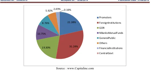
Source : www.Capitaline.com
Figure 1: Shareholding pattern of HDFC Bank (As at 31st March 2018)
2. REVIEW OF LITERATURE:
A plentiful amount of research has been undertaken in numerous disciplines or subjects that involve ARIMA methodology for the purpose of forecasting the future value(s) of a given variable. To discuss a few, Gay (2016) made an effort to investigate the relationship of macroeconomic variables on stock returns of BRIC countries that include Brazil, Russia, India and China. He made use of the Box-Jenkins method to serve the purpose. The factors taken into account were the exchange rates and the oil prices. No statistically significant association was found to be there between the given macroeconomic factors and stock returns for any of the BRIC economies. Moreover, no significant link was identified of stock return with its lagged values for any of the four countries. Similarly, Manoj and Madhu (2014) used the Box-Jenkins approach to predict the production of sugarcane in India. They found that the model was able to predict future production of sugarcane for almost five years. The most suitable ARIMA configuration for sugarcane was found to be ARIMA (2, 1, 0). Hamjah (2014) also employed ARIMA for anticipating rice production in Bangladesh. He made a comparison between the actual data of rice production and the predicted series and found that the model had a very good forecasting ability in the short run. Guha (2016) anticipated gold prices in India using ARIMA model in order to give insinuations to the investors about when, and when not, to buy gold. Jadhav, Reddy and Gaddi (2017) used ARIMA for predicting the prices of farms and then further used the same for major crops in the Karnataka state of India, namely the Paddi, Ragi and Maize. They took the data from 2002 to 2016 and found that the model had a very strong power to estimate values for the future. On the basis of this, they also forecasted the 2020 prices of the crops. Mondal, Shit and Goswami (2014) employed a sector-specific analysis of Indian stocks using ARIMA model. They conducted a study on the capability of the model using fifty six Indian stocks from various sectors. They found that the model correctly predicted stock prices to the extent of 85% for all sectors. Banerjee (2014) also used ARIMA to predict future Indian stock market index and found the model very accurate in short-term forecasting. Some Pakistani researchers also made use of ARIMA technique to forecast different time series variables. For instance, Zakria and Muhammad (2009)
used the model predict the future population of the country of Pakistan. They found out that if the country’s population continues to grow at the same rate, there are expected to be 230.68 million people in the country by 2027. The different statistical bureaus of Pakistan, on the other hand, have estimated the country’s population to reach 229 million by 2025. Hence, they concluded that the model worked well for predicting their variable of interest. In another study, Farooqi (2014) used ARIMA for predicting the imports and exports of Pakistan. They took the data from 1947 to 2013 and found that ARIMA (2, 2, 2) and ARIMA (1, 2, 2) worked better for predicting both imports and exports. Similarly, Saeed, Saeed, Zakria and Bajwa (2000) attempted to anticipate the production of wheat in Pakistan using the ARIMA model. They found in the diagnostic checking stage of their study that ARIMA (2, 2, 1) was most appropriate for the estimation of wheat production. They believed that the findings of the study would prove helpful for the concerned persons to foretell in advance the requirements of imports and exports of grain storage. In the same manner, Khan, Khan, Shaikh, Lodhi and Jilani (2015) also employed ARIMA model for predicting rice production in Pakistan. The data related to rice production was taken from 1993 to 2015. The diagnostic checking showed ARIMA (2, 1, 1) to be the most suitable ARIMA configuration for estimating rice production in Pakistan.
21.38%
31.24% 19.30%
10.75% 8.76%
5.92%2.49% 0.16%
Promoters
ForeignInstitutions
GDR
NBanksMutualFunds
GeneralPublic
Others
FinancialInstitutions
3. The ARIMA Model:
ARIMA model was introduced by statisticians George Box and Gwilym Jenkins in their book ‘Time Series Analysis: Forecasting and Control’ (Box & Jenkins, 1970). This method is suitable for time series of medium to longer length. According to Chatfield (1996), there should be at least 50 observations for ARIMA model to work. Many of the other researchers argue that the number of observations should be larger than 100 for the model to give better results. The model predicts future values of a time series on the basis of its past values and on the basis of the past values of error term. The foremost difficulty in ARIMA modeling is to identify how many lagged values of a variable as well as the error term effectively forecast the current, and future, value of the variable. The developers of the model, Box and Jenkins, have emphasized on keeping the model simple and condensed. A lengthy model which includes a larger number of regressors would be a better forecast but at the cost of decreasing degrees of freedom. The two scientists proposed a three-stage model for predicting a given time series. Therefore, the model is also popularly known as the Box-Jenkins methodology; although the econometric term for this type of model prediction is called the ARIMA modeling.
The four stages of the Box-Jenkins model are (a) identification of the model,
(b) model estimation, (c) diagnostic checking, and (d) forecasting.
Firstly we inspects plots of the autocorrelation function (ACF) and the partial autocorrelation function (PACF) simultaneously to check for patterns such as spikes, exponential decay or damped sinewave etc. Through this process, the most suitable ARIMA configuration, including the number of autoregressive processes (i.e., the AR) influencing a given time series variable, the number of moving average processes (i.e., the MA) and the number of times the series should be differenced in order to render it stationary (i.e., the d), for the time series is identified (Asteriou, 2007). This could also be done using function “auto.arima” . And then ADF (Augmented-Dickey Fuller Test) is conducted to know whether the data is Stationary or not. if data is non-stationary then In RStudio the series is made stationarity by taking the difference of the logged value of prices Then after selecting the best model from the ARIMA model the residuals testing is being conducted through Box.test to know whether the errors are Independently Identically distributed or not. At last the forecasting, the next or the future value of the time series is mathematically computed to see how close the forecasted value is with the actual value. This also gives calculation of the error term.
4. Research Methodology:
The study deals with analysis of a univariate time series. In case of time series analysis it is better the variables selected forstudy extracts the information from the variable itself. Therefore, , the autoregressive integrated moving average (ARIMA) model, also popularly known as the
Box-Jenkins methodology has been employed in the study. The general configuration for an ARIMA process as taken up from Asteriou and Hall (2007) is:
Yt= φ1Yt-1 + φ2Yt-2 + - - - + φpYt-p + εt + θ1εt-1 + θ2εt-2 + - - - + θqεt-q
Where, Yt is the predicted value of the variable,
Yt-1, Yt-2, - - - , Yt-p are the lagged values of the dependent variable or the autoregressive terms,
εt is the error term,
εt-1, εt-2, - - - , εt-q are the lagged values of the error or the moving average terms, and
φ and θ are the coefficients or slopes of the regressors.
5. Analysis:
Trading Periods
Figure2: Non-Stationary Share Prices of HDFC Bank
The above graph shows the closing prices of HDFC bank from 1.04.2008 to 31.03.2018.There has been a steady growth in the price. No major downfall has been seen in the period of study. However the data is non-stationary as it is not close to mean. The stationarity of the data was also checked through ADF Test.
Table1: Augmented Dickey Fuller Test for HDFC Stock Price
Null Hypothesis: HDFC has a unit root Exogenous: Constant
Lag Length: 0 (Automatic - based on SIC, maxlag=26)
t-Statistic Prob.* Augmented Dickey-Fuller test statistic 1.721973 0.9997 Test critical values: 1% level -3.432801
5% level -2.862509
10% level -2.567331
*MacKinnon (1996) one-sided p-values. Augmented Dickey-Fuller Test Equation Dependent Variable: D(HDFC)
Method: Least Squares Date: 07/26/19 Time: 20:51
Sample (adjusted): 4/02/2008 3/28/2018 Included observations: 2472 after adjustments
Variable Coefficient Std. Error t-Statistic Prob.
HDFC(-1) 0.000753 0.000437 1.721973 0.0852
C 0.084074 0.389151 0.216043 0.8290
R-squared 0.001199 Mean dependent var 0.659312 Adjusted R-squared 0.000795 S.D. dependent var 9.928393 S.E. of regression 9.924448 Akaike info criterion 7.428688
Sum squared resid 243281.8 Schwarz criterion 7.433391 Log likelihood -9179.859 Hannan-Quinn criter. 7.430397 F-statistic 2.965190 Durbin-Watson stat 1.953598 Prob(F-statistic) 0.085200
When the stationarity of the data was checked through ADF Test in table 4.1 it was concluded that data is Non-Stationary at level as the p value of the result obtained is greater than 0.05 and the value of Durbin-Watson comes out to be 1.95.
In order to induce stationarity, therefore, natural logarithms have been employed for stock prices and then the change in the log of stock prices, i.e., the first difference, has been taken into account and again the stationarity of the data was tested.
Differencing is simple operation that involves calculating consecutive changes in the values of the data series which means that the values of series fluctuate randomly around zero (average level).
Table2: Augmented Dickey-Fuller Test for Logged Differenced Stock Prices
Null Hypothesis: D(HDFC) has a unit root Exogenous: Constant
Lag Length: 0 (Automatic - based on SIC, maxlag=26)
t-Statistic Prob.*
Augmented Dickey-Fuller test statistic -48.45770 0.0001
Test critical values: 1% level -3.432802
5% level -2.862509
10% level -2.567331
*MacKinnon (1996) one-sided p-values. Augmented Dickey-Fuller Test Equation Dependent Variable: D(HDFC,2) Method: Least Squares
Date: 07/26/19 Time: 20:50
Sample (adjusted): 4/03/2008 3/28/2018 Included observations: 2471 after adjustments
Variable Coefficient Std. Error t-Statistic Prob.
D(HDFC(-1)) -0.974914 0.020119 -48.45770 0.0000
C 0.641866 0.200187 3.206333 0.0014
As the P-value is less than 0.05 and the value of Durbin Watson stat comes out to be 1.99. Hence it was concluded that the data is stationary at First Difference i.e. I(1).
After stationarity in the given time series has been achieved through logged differencing, we move on to apply the Box-Jenkins methodology. Box–Jenkins modeling has been successfully applied in various stock markets activities. These models allow investors who have data only from past years such as price shares, to forecast future prices once without having to search for other related time series data which are related with the time series that they study. The first step is the identification of the appropriate model which is being done through R studio using auto arima. Results Obtained were:
Table3: Selecting the Best ARIMA model
In the aforementioned section, it was found that the most suitable ARIMA configuration for forecasting HDFC’s prices is ARIMA (1, 0, 2). This implies that daily stock prices of HDFC can be predicted by taking into account one-day previous stock prices and two-one-day previous error term. Hence, mathematically, the following ARIMA model is to be employed:
Yt= µ + φ1Yt-1 + εt +θ1εt-1+ θ2εt-2
As per the results obtained the Equation comes out to be: Yt = 0.5493 Yt-1 -0.5042 εt-1 -0.0844 εt-2
Residuals are an important part of the study and therefore the stationarity of the residuals were checked through Box-Ljung Test.
Autocorrelation is used to measure the dependence of a variable on its past values. With this test we aim to determine whether the serial correlation coefficients are statistical significant (different from zero). The hypothesis of weak efficiency should be rejected if stock returns are serially correlated. The Box-Ljung Test is used, based on autocorrelation coefficients. Autocorrelation coefficients define the linear correlation between two observations of the returns time series. The Q-statistic is asymptotically distributed as a χ2 variable with degrees of freedom equal to the number of autocorrelations. Under this test, the null and alternative hypotheses are:
H0: No autocorrelation exist in the data. H1: Autocorrelation exist in the data .
Table4: Stationarity of Residuals
From the table 4 it can be seen that data does not contain unit root as p value is greater than 0.05 which means that Null hypothesis is accepted which means that there is no auto correlation between residuals. Hence it was concluded
ARIMA(1,0,2) with non-zero mean
Coefficients:
ar1 ma1 ma2 mean 0.5493 -0.5042 -0.0844 8e-04 s.e. 0.1611 0.1614 0.0201 3e-04
sigma^2 estimated as 0.0002996: log likelihood=6522.23 AIC=-13034.45 AICc=-13034.43 BIC=-13005.39
Box-Ljung test
data: rm1
that residuals are stationary. Therefore after selection of best model and checking the stationarity of residuals the forecasted value for next 10 working days were obtained.
Table5:Forecasted values of HDFC stocks on basis of fitted ARIMA
From the table 5 it can be seen that data does not contain unit root as p value is greater than 0.05 which means that Null hypothesis is accepted which means that there is no auto correlation between residuals. Hence it was concluded that residuals are stationary. Therefore after selection of best model and checking the stationarity of residuals the forecasted value for next 10 working days were obtained. And then the forecasted value was compared with the actual values and the difference between both the values was considered as forecasted error.
Table6:Comparison of Actual Prices and Forecasted Prices of HDFC stocks on basis of fitted ARIMA
Date Actual Price Forecasted Price Forecasted
Error(Rs.)
Forecasted Error(%)
02.04.2018 1930.45 1892.201 -38.249 -1.98135
03.04.2018 1916.10 1892.904 -23.196 -1.21058
04.04.2018 1884.80 1893.607 8.807 0.467264
05.04.2018 1907.70 1894.309 -13.391 -0.70194
06.04.2018 1922.70 1895.012 -27.688 -1.44006
09.04.2018 1938.50 1895.715 -42.785 -2.20712
10.04.2018 1919.10 1896.417 -22.683 -1.18196
11.04.2018 1916.25 1897.120 -19.13 -0.9983
12.04.2018 1926.30 1897.823 -28.477 -1.47833
13.04.2018 1928.05 1898.526 -29.524 -1.53129
5. CONCLUSION:
Prediction has always been a challenge for scientists in most of the disciplines. When it comes to financial theory, the process of speculation becomes even more susceptible as there are normally too many aspects or factors that need to be considered for actual forecasting. Some theorists, therefore, prefer to forecast the current (and/or future) price of a time series on the basis of its past values as well as the past values of the disturbance term. This concept, popularly known as the Box-Jenkins method and technically as the ARIMA method, was also employed in the current study. From the findings of the study, it has been construed that ARIMA has a very good capacity to forecast future values in the short run. The long-term prediction using lagged values of a variable makes only a little sense. As a policy implication, the autoregressive integrated moving average model can be helpful to stock market investors as a clue to anticipate whether the stocks that they have invested in are likely to move in upward direction, or vice versa, in the near future. When the actual values were compared with the predicted value it was observed that on all the days the forecasted value was underestimated except on 3rd day i.e. 03.04.2019 where the value was overestimated byRs.8.807. When the
percentage of standard error was calculated then it was observed that the value was overestimated around 2% except on 3rd day i.e. 03.04.2019 where the value was overestimated by 0.46%
REFERENCES:
1. Box, G. E., & Pierce, D. A. (1970). Distribution of residual autocorrelations in autoregressive-integrated moving average time series models. Journal of the American statistical Association, 65(332), 1509-1526.
2. Khan, K., Khan, Gulawar., Shaikh, S. A., Lodhi, A. S., & Jilani, G. (2015). ARIMA Modeling for Forecasting of Rice Production: A Case Study of Pakistan. Lasbela University Journal of Sciences and Technology, 4(1), 117-120.
3. Manoj, K., & Madhu, A. (2014). An Application of Time Series ARIMA Forecasting Model for Predicting Sugarcane Production in India. Studies in Business and Economics, 9(1), 81-90
4. Emang, D. et al., (2010). Forecasting with Univariate Time Series Models: A Case of Export Demand for Peninsular Malaysia’s Moulding and Chipboard, Journal of Sustainable Development, 3(3), pp: 157-161 5. Bhunia, A. (2013). Cointegration and Causal Relationship among Crude Price, Domestic Gold Price and
Financial Variables: An Evidence of BSE and NSE. Journal of Contemporary Issues in Business Research , 2 (1), 01-10.
6. Husin, M. M. (2013). Efficiency of Monetary Policy Transmission Mechanism via Profit Rate Channel for Islamic Banks in Malaysia. Journal of Contemporary Issues in Business Research , 2 (2), 44-55.
7. Kennedy, P. (2000). Macroeconomic Essentials:Understanding economics in the news. Massachusetts Institute of Technology.