Markov Properties for Linear Causal Models with Correlated Errors
Changsung Kang [email protected]
Jin Tian [email protected]
Department of Computer Science Iowa State University
Ames, IA 50011, USA
Editor: Andre Elisseeff
Abstract
A linear causal model with correlated errors, represented by a DAG with bi-directed edges, can be tested by the set of conditional independence relations implied by the model. A global Markov property specifies, by the d-separation criterion, the set of all conditional independence relations holding in any model associated with a graph. A local Markov property specifies a much smaller set of conditional independence relations which will imply all other conditional independence relations which hold under the global Markov property. For DAGs with bi-directed edges associated with arbitrary probability distributions, a local Markov property is given in Richardson (2003) which may invoke an exponential number of conditional independencies. In this paper, we show that for a class of linear structural equation models with correlated errors, there is a local Markov property which will invoke only a linear number of conditional independence relations. For general linear models, we provide a local Markov property that often invokes far fewer conditional independencies than that in Richardson (2003). The results have applications in testing linear structural equation models with correlated errors.
Keywords: Markov properties, linear causal models, linear structural equation models, graphical
models
1. Introduction
Linear causal models called structural equation models (SEMs) are widely used for causal reasoning in social sciences, economics, and artificial intelligence (Goldberger, 1972; Bollen, 1989; Spirtes et al., 2001; Pearl, 2000). One important problem in the applications of linear causal models is test-ing a hypothesized model against the given data. While the conventional method involves maximum likelihood estimation of the covariance matrix, an alternative approach has been proposed recently which involves testing for the conditional independence relationships implied by the model (Spirtes et al., 1998; Pearl, 1998; Pearl and Meshkat, 1999; Pearl, 2000; Shipley, 2000, 2003). The advan-tages of using this new test method instead of the traditional global fitting test have been discussed in Pearl (1998), Shipley (2000), McDonald (2002) and Shipley (2003). The method can be applied in small data samples and it can test “local” features of the model.
DAG, often called a global Markov property for the DAG, can be read by the d-separation crite-rion (Pearl, 1988). However, it is not necessary to test for all the independencies implied by the model as a subset of those independencies may imply all others. A local Markov property specifies a much smaller set of conditional independence relations which will imply (using the laws of prob-ability) all other conditional independence relations that hold under the global Markov property. A well-known local Markov property for DAGs is that each variable is conditionally independent of its non-descendants given its parents (Lauritzen et al., 1990; Lauritzen, 1996). Based on this local Markov property, Pearl and Meshkat (1999) and Shipley (2000) proposed testing methods for linear SEMs without correlated errors that involve at most one conditional independence test for each pair of variables.
On the other hand, the path diagrams for linear SEMs with correlated errors are DAGs with bi-directed edges (↔) where bi-directed edges are used to represent correlated errors. A DAG with bi-directed edges is called an acyclic directed mixed graph (ADMG) in Richardson (2003). The set of all conditional independence relations encoded in an ADMG can still be read by (a natural extension of) the d-separation criterion (called m-separation in Richardson, 2003) which provides the global Markov property for ADMGs (Spirtes et al., 1998; Koster, 1999; Richardson, 2003). A local Markov property for ADMGs is given in Richardson (2003), which, in the worst case, may invoke an exponential number of conditional independence relations, a sharp difference with the local Markov property for DAGs, where only one conditional independence relation is associated with each variable. Shipley (2003) suggested a method for testing linear SEMs with correlated errors but the method may or may not, depending on the actual models, be able to find a subset of conditional independence relations that imply all others.
In this paper, we seek to improve the local Markov property given in Richardson (2003) for linear SEMs with correlated errors. The local Markov property in Richardson (2003) is applicable for ADMGs associated with arbitrary probability distributions. Specifically, only semi-graphoid axioms which must hold in all probability distributions (Pearl, 1988) are used in showing that the set of conditional independence relations specified by the local Markov property will imply all those specified by the global Markov property. On the other hand, in linear SEMs, variables are assumed to have normal distributions, and it is known that normal distributions also satisfy the so-called composition axiom. Therefore, in this paper, we look for local Markov properties for ADMGs associated with probability distributions that satisfy the composition axiom. We will show that for a class of ADMGs, the local Markov property will invoke only one conditional independence relation for each variable, and therefore testing for the corresponding linear SEMs will involve at most one conditional independence test for each pair of variables. For general ADMGs, we provide a procedure that reduces the number of conditional independencies invoked by the local Markov property given in Richardson (2003), and therefore reduces the complexity of testing linear SEMs with correlated errors.
The paper is organized as follows. In Section 2, we introduce linear SEMs, give basic notation and definitions, and present the local Markov property developed in Richardson (2003). In Section 3, we show that for a class of ADMGs, there is a local Markov property for probability distributions satisfying the composition axiom that invokes only a linear number of conditional independence relations. We also show a local Markov property that may involve fewer conditioning variables. In Section 4, we consider general ADMGs (for probability distributions satisfying the composition axiom) and show a local Markov property that invokes fewer conditional independencies than that in Richardson (2003). Section 5 concludes the paper.
2. Preliminaries and Motivation
In this section, we give basic definitions and introduce some relevant concepts.
2.1 Linear Causal Models
The SEM technique was developed by geneticists (Wright, 1934) and economists (Haavelmo, 1943) for assessing cause-effect relationships from a combination of statistical data and qualitative causal assumptions. It is an important causal analysis tool widely used in social sciences, economics, and artificial intelligence (Goldberger, 1972; Duncan, 1975; Bollen, 1989; Spirtes et al., 2001). For a review of SEMs and causality we refer to Pearl (1998).
In an SEM, the causal relationships among a set of variables are often assumed to be linear and expressed by linear equations. Each equation describes the dependence of one variable in terms of the others. For example, an equation
Y =aX+ε (1)
represents that X may have a direct causal influence on Y and that no other variables have (direct) causal influences on Y except those factors (represented by the error termεtraditionally assumed to have normal distribution) that are omitted from the model. The parameter a quantifies the (direct) causal effect of X on Y . An equation like (1) with a causal interpretation represents an autonomous causal mechanism and is said to be structural.
As an example, consider the following model from Pearl (2000) that concerns the relations between smoking (X ) and lung cancer (Y ), mediated by the amount of tar (Z) deposited in a person’s lungs:
X=ε1,
Z=aX+ε2,
Y =bZ+ε3.
X
Smoking
Z
T a r in l u ngs
Y
C a nc e r
a b
Figure 1: Causal diagram illustrating the effect of smoking on lung cancer
cancer (Cov(ε1,ε3)6=0), but the genotype nevertheless has no effect on the amount of tar in the lungs except indirectly (through smoking). Often, it is illustrative to express our qualitative causal assumptions in terms of a graphical representation, as shown in Figure 1.
We now formally define the model that we will consider in this paper. A linear causal model (or
linear SEM) over a set of random variables V={V1, . . . ,Vn}is given by a set of structural equations of the form
Vj=
∑
icjiVi+εj, j=1, . . . ,n, (2)
where the summation is over the variables in V judged to be immediate causes of Vj. cji, called a
path coefficient, quantifies the direct causal influence of Vi on Vj. εj’s represent “error” terms due to omitted factors and are assumed to have normal distribution. We consider recursive models and assume that the summation in (2) is for i< j, that is, cji=0 for i≥ j.
We denote the covariances between observed variables σi j =Cov(Vi,Vj), and between error termsψi j=Cov(εi,εj). We denote the following matrices,Σ= [σi j],Ψ= [ψi j], and C= [ci j]. The parameters of the model are the non-zero entries in the matrices C andΨ. A parameterization of the model assigns a value to each parameter in the model, which then determines a unique covariance matrixΣgiven by (see, for example, Bollen, 1989)
Σ= (I−C)−1Ψ((I−C)t)−1.
The structural assumptions encoded in the model are the zero path coefficients and zero error covariances. The model structure can be represented by a DAG G with (dashed) bi-directed edges (an ADMG), called a causal diagram (or path diagram), as follows: the nodes of G are the variables
V1, . . . ,Vn; there is a directed edge from Vito Vj in G if Vi appears in the structural equation for Vj, that is, cji6=0; there is a bi-directed edge between Viand Vjif the error termsεiandεjhave non-zero correlation. For example, the smoking-and-lung-cancer SEM is represented by the causal diagram in Figure 1, in which each directed edge is annotated by the corresponding path coefficient.
We note that linear SEMs are often used without explicit causal interpretation. A linear SEM in which error terms are uncorrelated consists of a set of regression equations. Note that an equation as given by (2) is a regression equation if and only ifεj is uncorrelated with each Vi(Cov(Vi,εj) =0). Hence, an equation in an SEM with correlated errors may not be a regression equation. Linear SEMs provide a more powerful way to model data than the regression models taking into account correlated error terms.
2.2 Model Testing and Markov Properties
can be read from the causal diagram by the d-separation criterion as defined in the following.1 A
path between two vertices Vi and Vj in an ADMG consists of a sequence of consecutive edges of any type (directed or bi-directed). A vertex Vi is said to be an ancestor of a vertex Vj if there is a path Vi → · · · →Vj. A non-endpoint vertex W on a path is called a collider if two arrowheads on the path meet at W , that is,→W ←, ↔W ↔, ↔W ←,→W ↔; all other non-endpoint vertices on a path are non-colliders, that is,←W →,←W←,→W→,↔W→,←W↔. A path between vertices Viand Vj in an ADMG is said to be d-connecting given a set of vertices Z if
1. every non-collider on the path is not in Z, and
2. every collider on the path is an ancestor of a vertex in Z.
If there is no path d-connecting Viand Vjgiven Z, then Viand Vjare said to be d-separated given Z. Sets X and Y are said to be d-separated given Z, if for every pair Vi, Vj, with Vi∈X and Vj∈Y , Vi and Vjare d-separated given Z. Let I(X,Z,Y)denote that X is conditionally independent of Y given
Z. The set of all the conditional independence relations encoded by a causal diagram G is specified
by the following global Markov property.
Definition 1 (The Global Markov Property (GMP)) A probability distribution P is said to satisfy
the global Markov property for G if for arbitrary disjoint sets X,Y,Z with X and Y being nonempty,
(GMP) X is d-separated from Y given Z in G=⇒I(X,Z,Y).
The global Markov property typically involves a vast number of conditional independence relations and it is possible to test for a subset of those independencies that will imply all others. A local Markov property specifies a much smaller set of conditional independence relations which will imply by the laws of probability all other conditional independence relations that hold under the global Markov property. For example, a well-known local Markov property for DAGs is that each variable is conditionally independent of its non-descendants given its parents. The causal diagram for a linear SEM with correlated errors is an ADMG and a local Markov property for ADMGs is given in Richardson (2003).
Note that in linear SEMs, the conditional independence relations will correspond to zero partial correlations (Lauritzen, 1996):
ρViVj.Z=0⇐⇒I({Vi},Z,{Vj}).
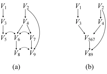
As an example, for the linear SEM with the causal diagram in Figure 2, if we use the local Markov property in Richardson (2003), then we need to test for the vanishing of the following set of partial correlations (for ease of notation, we writeρi j.Zto denoteρViVj.Z):
{ρ21,ρ32.1,ρ43.2,ρ41.2,ρ54.3,ρ52.3,ρ51.3,ρ64.53,ρ62.53,ρ61.53,ρ64.3,ρ62.3,ρ61.3,ρ72.6543, ρ71.6543,ρ72.643,ρ71.643,ρ75.4,ρ73.4,ρ72.4,ρ71.4}. (3) The local Markov property in Richardson (2003) is valid for any probability distributions. In fact, the equivalence of the global and local Markov properties is proved using the following so-called semi-graphoid axioms (Pearl, 1988) that probabilistic conditional independencies must sat-isfy:
V5 V6 V7
V3 V4
V1 V2
Figure 2: A causal diagram
• Symmetry
I(X,Z,Y)⇐⇒I(Y,Z,X).
• Decomposition
I(X,Z,Y∪W) =⇒I(X,Z,Y)& I(X,Z,W).
• Weak Union
I(X,Z,Y∪W) =⇒I(X,Z∪W,Y).
• Contraction
I(X,Z,Y)& I(X,Z∪Y,W) =⇒I(X,Z,Y∪W).
where X , Y , Z, and W are disjoint sets of variables.
On the other hand, in linear SEMs the variables are assumed to have normal distributions, and normal distributions also satisfy the following composition axiom:
• Composition
I(X,Z,Y)& I(X,Z,W) =⇒I(X,Z,Y∪W).
Therefore, we expect a local Markov property for linear SEMs to invoke fewer conditional inde-pendence relations than that for arbitrary distributions. In this paper, we will derive reduced local Markov properties for linear SEMs by making use of the composition axiom. As an example, for the linear SEM in Figure 2, a local Markov property which we will present in this paper (see Sec-tion 3.3) says that we only need to test for the vanishing of the following set of partial correlaSec-tions:
{ρ21,ρ32,ρ43,ρ41,ρ54,ρ52,ρ51.3,ρ64,ρ62,ρ61.3,ρ75,ρ73,ρ71,ρ72.4}.
The number of tests needed and the size of the conditioning set Z are both substantially reduced compared with (3), thus leading to a more economical way of testing the given model.
2.3 A Local Markov Property for ADMGs
In this section, we describe the local Markov property for ADMGs associated with arbitrary proba-bility distributions presented in Richardson (2003). In this paper, this Markov property will be used as an important tool to prove the equivalence of our local Markov properties and the global Markov property.
V5 V6 V7 V3 V4
V8 V9 V1 V2
V56 7 V3 V4
V8 9 V1 V2
(a ) (b )
Figure 3: An ADMG and its compressed graph
{Y|Y → · · · →X in G or Y =X}is the set of ancestors of X . And deG(X)≡ {Y|Y ← · · · ←X in
G or Y =X}is the set of descendants of X . These definitions will be applied to sets of vertices, so that, for example, paG(A)≡ ∪X∈ApaG(X), spG(A)≡ ∪X∈AspG(X), etc.
Definition 2 (C-component) A c-component of G is a maximal set of vertices in G such that any
two vertices in the set are connected by a path on which every edge is of the form↔; a vertex that is not connected to any bi-directed edge forms a c-component by itself.
For example, the ADMG in Figure 3 (a) is composed of 6 c-components{V1}, {V2}, {V3},{V4},
{V5,V6,V7}and{V8,V9}. The district of X in G is the c-component of G that includes X . Thus, disG(X)≡ {Y|Y ↔ · · · ↔X in G or Y =X}.
For example, in Figure 3 (a), we have disG(V5) ={V5,V6,V7}and disG(V8) ={V8,V9}. A set A is said to be ancestral if it is closed under the ancestor relation, that is, if anG(A) =A. Let GAdenote the induced subgraph of G on the vertex set A, formed by removing from G all vertices that are not in A, and all edges that do not have both endpoints in A.
Definition 3 (Markov Blanket)2 If A is an ancestral set in an ADMG G, and X is a vertex in A that has no children in A then the Markov blanket of vertex X with respect to the induced subgraph
on A, denoted mb(X,A)is defined to be
mb(X,A)≡paGA(disGA(X))∪(disGA(X)\ {X}).
For example, for an ancestral set A=anG({V5,V6}) ={V1,V2,V3,V4,V5,V6}in Figure 3 (a), we have mb(V5,A) ={V3,V4,V6}.
An ordering (≺) on the vertices of G is said to be consistent with G if X ≺Y ⇒Y∈/anG(X). Given a consistent ordering≺, let preG,≺(X)≡ {Y|Y ≺X or Y =X}.
Definition 4 (The Ordered Local Markov Property (LMP,≺)) A probability distribution P
sat-isfies the ordered local Markov property for G with respect to a consistent ordering≺, if, for any X and ancestral set A such that X∈A⊆preG,≺(X),
(LMP,≺) I({X},mb(X,A),A\(mb(X,A)∪ {X})). (4)
Theorem 5 (Richardson, 2003) If G is an ADMG and≺is a consistent ordering, then a probability distribution P satisfies the ordered local Markov property for G with respect to≺if and only if P satisfies the global Markov property for G.
We will write (GMP)⇐⇒(LMP,≺) to denote the equivalence of the two Markov properties. There-fore the (smaller) set of conditional independencies specified in the ordered local Markov erty will imply all other conditional independencies which hold under the global Markov prop-erty. It is possible to further reduce the number of conditional independence relations in the or-dered local Markov property. An ancestral set A, with X ∈A⊆preG,≺(X) is said to be
maxi-mal with respect to the Markov blanket mb(X,A) if, whenever there is a set B such that A⊆B⊆
preG,≺(X)and mb(X,A) =mb(X,B), then A=B. For example, suppose that we are given an
or-dering≺: V1≺V2≺V3≺V4≺V5≺V6≺V7≺V8≺V9 for the graph G in Figure 3 (a). While an ancestral set A=anG({V3,V6,V7}) ={V1,V2,V3,V4,V6,V7}is maximal with respect to the Markov blanket mb(V7,A) ={V4,V6}, an ancestral set A0=anG({V6,V7}) ={V2,V4,V6,V7} is not. It was shown that we only need to consider ancestral sets A which are maximal with respect to mb(X,A)in the ordered local Markov property (Richardson, 2003). Thus, we will consider only maximal ances-tral sets A when we discuss (LMP,≺) for the rest of this paper. The following lemma characterizes maximal ancestral sets.
Lemma 6 (Richardson, 2003) Let X be a vertex and A an ancestral set in G with consistent ordering
≺such that X∈A⊆preG,≺(X). The set A is maximal with respect to the Markov blanket mb(X,A) if and only if
A=preG,≺(X)\deG(h(X,A))
where
h(X,A)≡spGdisGA(X)
\{X} ∪mb(X,A).
Even though we only consider maximal ancestral sets, the ordered local Markov property may still invoke an exponential number of conditional independence relations. For example, for a vertex
X , if disG(X)⊆preG,≺(X)and disG(X)has a clique of n vertices joined by bi-directed edges, then there are at least O(2n−1)different Markov blankets.
It should be noted that only the semi-graphoid axioms were used to prove Theorem 5 on the equivalence of the two Markov properties and no assumptions about probability distributions were made. Next we will show that the ordered local Markov property can be further reduced if we use the composition axiom in addition to the semi-graphoid axioms. The local Markov properties we obtained (in Sections 3 and 4) are not restricted to linear causal models in that they are actually valid for any probability distributions that satisfy the composition axiom.
3. Markov Properties for ADMGs without Directed Mixed Cycles
In this section, we introduce three local Markov properties for a class of ADMGs and show that they are equivalent to the global Markov property. Also, we discuss related work in maximal ancestral graphs and chain graphs. First, we give some definitions.
Definition 7 (Directed Mixed Cycle) A path is said to be a directed mixed path from X to Y if
X Y
Z W
Figure 4: Directed mixed cycles
For example, the path X→Z↔W→Y↔X in the graph in Figure 4 forms a directed mixed cycle.
In this section, we will consider only ADMGs without directed mixed cycles.
Definition 8 (Compressed Graph) Let G be an ADMG. The compressed graph of G is defined to be
the graph G0= (V0,E0), V0={VC|C is a c-component of G}, E0={VCi→VCj|there is an edge X→
Y in G such that X ∈Ci,Y∈Cj}.
Figure 3 shows an ADMG and its compressed graph. If there exists a directed mixed cycle in an ADMG G, there will be a cycle or a self-loop in the compressed graph of G. For example, if for two vertices X and Y in a c-component C of G there exists an edge X →Y , then the compressed graph
of G contains a self-loopy
VC. The following proposition holds.
Proposition 9 Let G be an ADMG. The compressed graph of G is a DAG if and only if G has no
directed mixed cycles.
3.1 The Reduced Local Markov Property
In this section, we introduce a local Markov property for ADMGs without directed mixed cycles which only invokes a linear number of conditional independence relations and show that it is equiv-alent to the global local Markov property.
Definition 10 (The Reduced Local Markov Property (RLMP)) Let G be an ADMG without
di-rected mixed cycles. A probability distribution P is said to satisfy the reduced local Markov property for G if
(RLMP) ∀X∈V, I({X},paG(X),V\f(X,G)) (5)
where f(X,G)≡paG(X)∪deG({X} ∪spG(X)).
The reduced local Markov property states that a variable is independent of the variables that are
neither its descendants nor its spouses’ descendants given its parents.
Theorem 11 If a probability distribution P satisfies the composition axiom and an ADMG G has
no directed mixed cycles, then
(GMP)⇐⇒(RLMP).
Proof:(GMP) =⇒(RLMP)
1. X ←β· · ·α
2. X → · · · →δ←∗ · · ·α
3. X ↔γ←∗ · · ·α
4. X ↔γ→ · · · →δ←∗ · · ·α
A symbol∗serves as a wildcard for an end of an edge. For example, ←∗represents both← and
↔. In case 1,β∈paG(X). In case 2, the colliderδis not an ancestor of a vertex in paG(X) (other-wise, there would be a cycle). In cases 3 and 4, neitherγnorδis an ancestor of a vertex in paG(X) (otherwise, there would be directed mixed cycles). In any case, the path is not d-connecting given
paG(X).
Proof:(RLMP) =⇒(GMP)
We will show that for some consistent ordering≺,(RLMP) =⇒(LMP,≺). Then, by Theorem 5, we have(RLMP) =⇒(GMP).
We construct a consistent ordering with the desired property as follows.
1. Construct the compressed graph G0of G.
2. Let ≺0 be any consistent ordering on G0. Construct a consistent ordering ≺ from ≺0 by
replacing each VC (corresponding to each c-component C of G) in≺0with the vertices in C (the ordering of the vertices in C is arbitrary).
We now prove that (RLMP) =⇒ (LMP,≺). Assume that a probability distribution P satisfies (RLMP). Consider the set of conditional independence relations invoked by (LMP,≺) for each vari-able X given in (4). First, observe that for any vertex Y in disGA(X), we have
A\(paG(Y)∪ {Y} ∪spG(Y))⊆V\f(Y,G),
since
A\(paG(Y)∪ {Y} ∪spG(Y))
=A\
paG(Y)∪ {Y} ∪spG(Y)∪deG({Y} ∪spG(Y))\({Y} ∪spG(Y))
(6)
=A\f(Y,G).
The equality (6) holds since the vertices in deG({Y} ∪spG(Y))\({Y} ∪spG(Y))do not appear in A (because of the way≺is constructed, no descendant of disGA(X)is in A). Thus, by (5), for all Y in
disGA(X), we have
I({Y},paG(Y),A\(paG(Y)∪ {Y} ∪spGA(Y))).
Let S1=paG(disGA(X))\paG(Y)and S2=A\(mb(X,A)∪ {X}). It follows that
S1⊆A\(paG(Y)∪ {Y} ∪spG(Y))and
Also, we have
S1∩S2=/0, since S1⊆mb(X,A). Therefore, for Y ∈disGA(X),
I({Y},paG(Y),S1∪S2) by decomposition
I({Y},paG(Y)∪S1,S2) by weak union
I(disGA(X),paG(disGA(X)),A\(mb(X,A)∪ {X})) by composition
I({X},paG(disGA(X))∪(disGA(X)\ {X}),
A\(mb(X,A)∪ {X})) by weak union.
Thus, we have
I({X},mb(X,A),A\(mb(X,A)∪ {X}))
by the definition of the Markov blanket of X with respect to A.
As an example, consider the ADMG G in Figure 3 (a) which has no directed mixed cycles. The graph in Figure 3 (b) is the compressed graph G0 of G described in the proof. From the ordering
≺0: V1≺V
2≺V3≺V4 ≺V567≺V89, we obtain the ordering ≺: V1 ≺V2≺V3≺V4≺V5 ≺V6≺
V7 ≺V8 ≺V9. The ordered local Markov property (LMP,≺) involves the following conditional independence relations:
I({V2},/0,{V1}), I({V3},{V1},{V2}),
I({V4},{V2},{V1,V3}), I({V5},{V3},{V1,V2,V4}),
I({V6},{V3,V4,V5},{V1,V2}), I({V6},{V4},{V1,V2,V3}),
I({V7},{V3,V4,V5,V6},{V1,V2}), I({V7},{V4,V6},{V1,V2,V3}),
I({V7},{V4},{V1,V2,V3,V5}), I({V8},{V6},{V1,V2,V3,V4,V5,V7}),
I({V9},{V2,V6,V7,V8},{V1,V3,V4,V5}), I({V9},{V2,V7},{V1,V3,V4,V5,V6}). (7) (RLMP) invokes the following conditional independence relations:
I({V1},/0,{V2,V4,V6,V7,V8,V9}), I({V2},/0,{V1,V3,V5}),
I({V3},{V1},{V2,V4,V6,V7,V8,V9}), I({V4},{V2},{V1,V3,V5}),
I({V5},{V3},{V1,V2,V4,V7,V9}), I({V6},{V4},{V1,V2,V3}),
I({V7},{V4},{V1,V2,V3,V5}), I({V8},{V6},{V1,V2,V3,V4,V5,V7}),
I({V9},{V2,V7},{V1,V3,V4,V5,V6}) (8) which, by Theorem 11, imply all the conditional independence relations in (7).
For the special case of graphs containing only bi-directed edges,3 Kauermann (1996) provides a local Markov property for probability distributions obeying the composition axiom as follows:
∀X∈V, I({X},/0,V\({X} ∪spG(X))). (9)
Since a graph containing only bi-directed edges is a special case of ADMGs without directed mixed cycles, the reduced local Markov property (RLMP) is applicable, and it turns out that (RLMP) reduces to (9) for graphs containing only bi-directed edges. Therefore (RLMP) includes the local Markov property given in Kauermann (1996) as a special case.
3.2 The Ordered Reduced Local Markov Property
The set of zero partial correlations corresponding to a conditional independence relation I(X,Z,Y) is
{ρViVj.Z=0|Vi∈X,Vj∈Y}.
Although (RLMP) gives only a linear number of conditional independence relations, the number of zero partial correlations may be larger than that invoked by (LMP,≺) in some cases. For example, 12 conditional independence relations in (7) involve 37 zero partial correlations while 9 conditional independence relations in (8) involve 41 zero partial correlations. In this section, we will show an ordered local Markov property such that at most one zero partial correlation is invoked for each pair of variables.
Definition 12 (C-ordering) Let G be an ADMG. A consistent ordering≺on the vertices of G is said to be a c-ordering if all the vertices in each c-component of G are consecutively ordered in≺.
For example, the ordering V1≺V2≺V3≺V4≺V5≺V6≺V7≺V8≺V9is a c-ordering on the vertices of G in Figure 3 (a). The following holds.
Proposition 13 There exists a c-ordering on the vertices of G if G does not have directed mixed
cycles.
We can easily construct a c-ordering from the compressed graph of G. We introduce the following Markov property.
Definition 14 (The Ordered Reduced Local Markov Property (RLMP,≺c)) Let G be an ADMG
without directed mixed cycles and≺cbe a c-ordering on the vertices of G. A probability distribution
P is said to satisfy the ordered reduced local Markov property for G with respect to≺cif
(RLMP,≺c) ∀X∈V,I({X},paG(X),preG,≺c(X)\({X} ∪paG(X)∪spG(X))). (10)
The ordered reduced local Markov property states that a variable is independent of its predecessors,
excluding its spouses, in a c-ordering given its parents. We now establish the equivalence of (GMP)
and (RLMP,≺c).
Theorem 15 If a probability distribution P satisfies the composition axiom and an ADMG G has
no directed mixed cycles, then for a c-ordering≺con the vertices of G,
Proof: (GMP)=⇒(RLMP,≺c)
The set preG,≺c(X)does not include any descendant of disG(X)since≺cis a c-ordering. We have
preG,≺c(X)\({X} ∪paG(X)∪spG(X))
=preG,≺c(X)\
{X} ∪paG(X)∪spG(X)∪deG({X} ∪spG(X))\({X} ∪spG(X))
=preG,≺c(X)\f(X,G)
⊆V\f(X,G).
Hence, (RLMP,≺c) follows from (RLMP).
Proof: (RLMP,≺c)=⇒(GMP)
We will show that (RLMP,≺c) =⇒ (LMP,≺c). Assume that a probability distribution P satisfies (RLMP,≺c). Let g(Y) =preG,≺c(Y)\({Y} ∪paG(Y)∪spG(Y)). Consider the set of conditional
independence relations invoked by (LMP,≺c) for each variable X given in (4) where A is maximal. By (10), for all Y in disGA(X), we have
I(Y,paG(Y),g(Y)). (11)
Let S1=paG(disGA(X))\paG(Y)and S2=A\(mb(X,A)∪ {X}). We have that
S1⊆g(Y).
Note that S2\g(Y)may be non-empty. Let S3=S2\g(Y). It suffices to show that
I(Y,paG(Y),S3),
which implies I(Y,paG(Y),S2)by composition. Then, the rest of the proof would be identical to that of Theorem 11.
We first characterize the vertices in S3. We will show that
S3= (preG,≺c(X)\preG,≺c(Y))\spG(disGA(X)). (12)
By Lemma 6, we have
S2=preG,≺c(X)\
deG(h(X,A))∪mb(X,A)∪ {X}
.
Since≺cis a c-ordering, no descendant of disG(X)will appear in A. Hence,
S2=preG,≺c(X)\
spG(disGA(X))∪paG(disGA(X))
.
To identify some common elements of S2and g(Y), we will reformulate S2and g(Y)as follows.
S2=
B\paG(disGA(X))
∪(disG(X)∩preG,≺c(X))\spG(disGA(X))
,
g(Y) =B\paG(Y)∪(disG(X)∩preG,≺c(Y))\({Y} ∪spG(Y))
where B=preG,≺c(X)\disG(X). This can be verified by noting that A1=A2\(A3∪A4) = (A11\
A2)∪(A12\A3)if A1=A11∪A12,A11∩A12=/0,A2⊆A11,A3⊆A12. From paG(Y)⊆paG(disGA(X)),
it follows that B\paG(disGA(X))⊆B\paG(Y)and
S3=S2\g(Y)
=(disG(X)∩preG,≺c(X))\spG(disGA(X))
\(disG(X)∩preG,≺c(Y))\({Y} ∪spG(Y))
.
We can rewrite the first part of this expression as follows.
(disG(X)∩preG,≺c(X))\spG(disGA(X))
=(disG(X)∩preG,≺c(Y))\spG(disGA(X))
∪(preG,≺c(X)\preG,≺c(Y))\spG(disGA(X))
.
From(disG(X)∩preG,≺c(Y))\spG(disGA(X))⊆(disG(X)∩preG,≺c(Y))\({Y} ∪spG(Y)), (12)
fol-lows. Thus, the vertices in S3 are those in the set preG,≺c(X)\preG,≺c(Y) and not in the set
spG(disGA(X)).
Now we are ready to prove I(Y,paG(Y),S3). For any Z∈S3, we have Y ≺Z and Z∈/spG(Y). Hence,
I({Z},paG(Z),g(Z)),
I({Z},paG(Z),{Y} ∪(paG(Y)\paG(Z))) by decomposition,
I({Z},paG(Z)∪paG(Y),{Y}) by weak union,
I({Y},paG(Y),paG(Z)\paG(Y)) by paG(Z)\paG(Y))⊆g(Y),(11) and decomposition,
I({Y},paG(Y),{Z}) by contraction and decomposition.
Therefore, by composition, I(Y,paG(Y),S3)holds.
(RLMP,≺c) invokes one zero partial correlation for each pair of nonadjacent variables. For example, for the ADMG G in Figure 3 (a) and a c-ordering≺c: V1≺V2≺V3≺V4≺V5≺V6≺V7≺
V8≺V9, (RLMP,≺c) invokes the following conditional independence relations:
I({V2},/0,{V1}), I({V3},{V1},{V2}),
I({V4},{V2},{V1,V3}), I({V5},{V3},{V1,V2,V4}),
I({V6},{V4},{V1,V2,V3}), I({V7},{V4},{V1,V2,V3,V5}),
I({V8},{V6},{V1,V2,V3,V4,V5,V7}), I({V9},{V2,V7},{V1,V3,V4,V5,V6}) (13) which involve 25 zero partial correlations while (7) involve 37 zero partial correlations.
3.3 The Pairwise Markov Property
previous sections, we focused on minimizing the number of zero partial correlations. We now take into account the size of the conditioning set Z in each zero partial correlation ρXY.Z. When the size of paG(X) for a vertex X in (RLMP,≺c) is large, it might be advantageous to use a different conditioning set with smaller size (if the equivalence of the Markov properties still holds). Pearl and Meshkat (1999) introduced a pairwise Markov property for DAGs (without bi-directed edges) which may involve fewer conditioning variables and thus lead to more economical tests. The result can be easily generalized to ADMGs with no directed mixed cycles.
Let d(X,Y)denote the shortest distance between two vertices X and Y , that is, the number of edges in the shortest path between X and Y . Two vertices X and Y are nonadjacent if X and Y are not connected by a directed nor a bi-directed edge.
Definition 16 (The Pairwise Markov Property (PMP,≺c)) Let G be an ADMG without directed
mixed cycles and≺c be a c-ordering on the vertices of G. A probability distribution P is said to
satisfy the pairwise Markov property for G with respect to≺c if for any two nonadjacent vertices
Vi,Vj,Vj≺cVi
(PMP,≺c) I({Vi},Zi j,{Vj})
where Zi jis any set of vertices such that Zi jd-separates Vifrom Vjand∀Z∈Zi j,d(Vi,Z)<d(Vi,Vj).
Note that, in ADMGs with no directed mixed cycles, there always exists such a Zi j for any two nonadjacent vertices. For example, the parent set of Vi always satisfies the condition for Zi j. If the empty set d-separates Vi from Vj, then the empty set is defined to satisfy the condition for Zi j. Therefore we can always choose a Zi j with the smallest size, providing a more economical way to test zero partial correlations.
Theorem 17 If a probability distribution P satisfies the composition axiom and an ADMG G has
no directed mixed cycles, then
(GMP)⇐⇒(PMP,≺c).
Proof: Noting that two vertices X and Y are adjacent if X ←Y , X →Y or X↔Y , the proof of
Theorem 1 by Pearl and Meshkat (1999) is directly applicable to ADMGs and it effectively proves
that (RLMP,≺c)⇐⇒(PMP,≺c). We do not reproduce the proof here.
As an example, for the ADMG G in Figure 3 (a) and a c-ordering≺c: V1≺V2≺V3≺V4≺V5≺
V6≺V7≺V8≺V9, the following conditional independence relations (for convenience, we combine the relations for each vertex that have the same conditioning set) can be given by (PMP,≺c):
I({V2},/0,{V1}), I({V3},/0,{V2}),
I({V4},/0,{V3,V1}), I({V5},/0,{V4,V2}),
I({V5},{V3},{V1}), I({V6},/0,{V3,V1}),
I({V6},{V4},{V2}), I({V7},/0,{V5,V3,V1}),
I({V7},{V4},{V2}), I({V8},{V6},{V7,V5,V4,V2}),
I({V8},/0,{V3,V1}), I({V9},{V2,V7},{V6,V4}),
I({V9},/0,{V5,V3,V1})
3.4 Relation to Other Work
In this section, we contrast the class of ADMGs without directed mixed cycles to maximal ancestral graphs and chain graphs in terms of Markov properties.
3.4.1 MAXIMALANCESTRALGRAPHS
It is easy to see that an ADMG without directed mixed cycles is a maximal ancestral graph (MAG) (Richardson and Spirtes, 2002). An ADMG is said to be ancestral if, for any edge X↔Y , X is not
an ancestor of Y (and vice versa). Note that an edge X↔Y and a directed path from X to Y (or Y to X ) form a directed mixed cycle. Hence, an ADMG without directed mixed cycles is ancestral. An
ancestral graph is said to be maximal if, for any pair of nonadjacent vertices X and Y , there exists a set Z⊆V\ {X,Y}that d-separates X from Y . From Theorem 17, it follows that an ADMG without directed mixed cycles is maximal. On the other hand, there exist MAGs which have directed mixed cycles (see Figure 4). Thus, the class of ADMGs without directed mixed cycles is a strict subclass of MAGs.
Richardson and Spirtes (2002, p.979) showed the following pairwise Markov property for a MAG G:
I({Vi},anG({Vi,Vj})\ {Vi,Vj},{Vj})
for any two nonadjacent vertices Viand Vj. Richardson and Spirtes (2002) proved that this pairwise Markov property implies the global Markov property assuming a Gaussian parametrization. This does not trivially imply our results in Section 3.3 and our results cannot be considered as a special case of the results on MAGs. The two pairwise Markov properties involve two different forms of conditioning sets. The pairwise Markov property for MAGs involves considerably larger condition-ing sets than our pairwise Markov property: the conditioncondition-ing set includes all ancestors of Viand Vj, which is undesirable for our purpose of using the zero partial correlations to test a model.
Also, it should be stressed that our results do not depend on a specific parameterization. We only require the composition axiom to be satisfied. In contrast, Richardson and Spirtes (2002) consider only Gaussian parameterizations. It requires further study whether the pairwise Markov property for MAGs can be generalized to the class of distributions satisfying the composition axiom.
In the next section, we consider general ADMGs and try to eliminate redundant conditional independence relations from (LMP,≺). The class of MAGs is clearly a (strict) subclass of ADMGs. Hence, given a MAG, we have two options: either we use the result in the next section or the pairwise Markov property for MAGs. Although the pairwise Markov property for MAGs gives fewer zero partial correlations (one for each nonadjacent pair of vertices), it is possible that in some cases we are better off using the result in the next section (because of the cost incurred by the large conditioning sets in the pairwise Markov property for MAGs). An example of this situation will be given in the next section.
3.4.2 CHAINGRAPHS
The graph that results from replacing bi-directed edges with undirected edges in an ADMG without directed mixed cycles is a chain graph. The class of chain graphs has been studied extensively (see Lauritzen, 1996, for a review).
Some Markov properties have been proposed for chain graphs. The first Markov property for chain graphs has been proposed by Lauritzen and Wermuth (1989) and Frydenberg (1990). An-dersson et al. (2001) have introduced another Markov property. These two Markov properties do not correspond to the Markov property for ADMGs. Let G be an ADMG without directed mixed cycles and G0be the chain graph obtained by replacing bi-directed edges with undirected edges. In general, the set of conditional independence relations given by the Markov property for G is not equivalent to that given by either of the two Markov properties for chain graphs. However, there are other Markov properties for chain graphs that correspond to the Markov property for ADMGs without directed mixed cycles (Cox and Wermuth, 1993; Wermuth and Cox, 2001, 2004).4
4. Markov Properties for General ADMGs
When an ADMG G has directed mixed cycles, (RLMP), (RLMP,≺c), and (PMP,≺c) are no longer equivalent to (GMP) while (LMP,≺) still is. In this section, we show that the number of conditional independence relations given by (LMP,≺) for an arbitrary ADMG that might have directed mixed cycles can still be reduced. We introduce a procedure to reduce (LMP,≺). We then give an example to illustrate the procedure.
4.1 Reducing the Ordered Local Markov Property
First, we introduce a lemma that gives a condition by which a conditional independence relation renders another conditional independence relation redundant.
Lemma 18 Given an ADMG G, a consistent ordering ≺ on the vertices of G and a vertex X , assume that a probability distribution P satisfies the global Markov property for GpreG,≺(X)\{X}. Let
A=preG,≺(X)and A0be a maximal ancestral set with respect to mb(X,A0)such that X ∈A0⊂A, A0∩disGA(X) =disGA0(X)and paG(disGA(X)\disGA0(X))⊆mb(X,A
0). Then,
I({X},mb(X,A),A\(mb(X,A)∪ {X})) (14)
implies
I({X},mb(X,A0),A0\(mb(X,A0)∪ {X})).
We define rdG,≺(X)to be the set of all A0 satisfying this condition.
Proof: First, we show the relationships among A,disGA(X), mb(X,A)and A
0,dis
GA0(X), mb(X,A0).
By Lemma 6, we have
A0=A\deGA(h(X,A
0)) (15)
where
h(X,A0)≡spGA
disGA0(X)
\{X} ∪mb(X,A0).
● X ● … ● … ● ● ● … ● ● … … …
T d i s ( )
' X A G
))
(
( d i s p a ' X A G G A ′ ) (
d e T
A
G
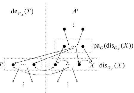
Figure 5: The relationship between A and A0 that satisfy the conditions in Lemma 18. The induced subgraph GA is shown. The vertices of GA are decomposed into two disjoint subsets deGA(T)and A
0.
disGA0(X)and h(X,A0)are subsets of disGA(X). Since disGA0(X)⊆ {X}∪mb(X,A
0)(by the definition
of the Markov blanket), disGA0(X)∩h(X,A
0) =/0. Thus, we can decompose the set dis
GA(X)into 3
disjoint subsets as follows.
disGA(X) =disGA0(X)∪h(X,A
0)∪B (16)
where
B≡disGA(X)\
disGA0(X)∪h(X,A
0).
We have
A0∩disGA(X) =A
0∩dis
GA0(X)∪h(X,A
0)∪B
=disGA0(X)∪B
since disGA0(X)⊆A
0,B⊆A0 and A0∩h(X,A0) = /0. From the assumption in Lemma 18 that A0∩
disGA(X) =disGA0(X), it follows that B= /0. Thus, from (16), we have
disGA(X)\disGA0(X) =h(X,A
0). (17)
Let T =disGA(X)\disGA0(X) =h(X,A
0). Then,
mb(X,A) =mb(X,A0)∪T∪paG(T)
=mb(X,A0)∪T (18)
since paG(T)⊆mb(X,A0)by our assumption. Thus A decomposes into
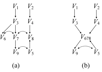
V6 V7 V8
V3 V4
V9 V5
V1 V2
V67 8
V3 V4
V9
V1 V2
(a ) (b )
V5
Figure 6: (a) An ADMG with directed mixed cycles (b) Illustration of the procedure GetOrdering. The modified graph after the first step is shown.
since deGA(T)⊆A and (15).
The key relationships among A,disGA(X),mb(X,A) and A
0,dis
GA0(X),mb(X,A0) are given by
(17)–(19). Figure 5 shows these relationships. We are now ready to prove that I({X},mb(X,A0),A0\
(mb(X,A0)∪ {X}))can be derived from I({X},mb(X,A),A\(mb(X,A)∪ {X})). From (18) and (19), it follows that
A\(mb(X,A)∪ {X}) = (A0∪deGA(T))\(mb(X,A
0)∪ {X} ∪T).
Since A0∩deGA(T) = /0,(mb(X,A
0)∪ {X})∩T = /0,mb(X,A0)∪ {X} ⊆A0 and T ⊆de
GA(T), we
have
A\(mb(X,A)∪ {X}) =A0\(mb(X,A0)∪ {X})∪deGA(T)\T
. (20)
Plugging (18) and (20) into (14), we get
I{X},mb(X,A0)∪T,A0\(mb(X,A0)∪ {X})∪deGA(T)\T
.
From the decomposition axiom, it follows that
I({X},mb(X,A0)∪T,A0\(mb(X,A0)∪ {X})). (21)
The last step is to remove T from the conditioning set to obtain I({X},mb(X,A0),A0\(mb(X,A0)∪ {X})). We claim that
I(T,mb(X,A0),A0\(mb(X,A0)∪ {X})). (22)
We first argue that T is d-separated from A0\(mb(X,A0)∪ {X})given mb(X,A0). Consider a vertex
t∈T and a vertexα∈A0\(mb(X,A0)∪ {X}). Note that for any bi-directed edge t↔βin GA,βis either in T or disGA0(X). There are only four possible cases for any path in GAfrom t toα.
1. t←γ· · ·α
3. t↔↔ · · · ↔δ←γ· · ·α
4. t↔↔ · · · ↔δ→ · · · →γ←∗ · · ·α
In case 1, γ∈mb(X,A0) since paG(T)⊆mb(X,A0). Thus, the path is not d-connecting. In case 2, γ is a descendant of t. Since mb(X,A0) does not contain any descendant of t, the path is not d-connecting. Case 3 is similar to case 1, but there are one or more bi-directed edges after t. δis either in T or disGA0(X). It follows thatγ∈mb(X,A
0), so the path is not d-connecting. Case 4 is
similar to case 2, but there are one or more bi-directed edges after t. Ifδis in T , the argument for case 2 can be applied. Ifδis in disGA0(X), then δ∈mb(X,A0), which implies that the path is not
d-connecting. This establishes that T is d-separated from A0\(mb(X,A0)∪ {X})given mb(X,A0). By the assumption that P satisfies the global Markov property for GpreG,≺(X)\{X}, (22) holds. Finally,
from (21),(22) and the contraction axiom, it follows that I({X},mb(X,A0),A0\(mb(X,A0)∪ {X})).
For example, consider the ADMG G in Figure 2 and a consistent ordering V1 ≺V2 ≺V3≺
V4≺V5≺V6 ≺V7. Assume that the global Markov property for GpreG,≺(V6) is satisfied. Let A=
{V1,V2,V3,V4,V5,V6,V7}and A0={V1,V2,V3,V4,V6,V7}. Then, disGA(V7) ={V5,V6,V7}, disGA0(V7) =
{V6,V7}, A0∩disGA(V7)={V6,V7}=disGA0(V7)and paG(disGA(V7)\disGA0(V7))={V3} ⊆ {V3,V4,V6}
= mb(V7,A0). Thus, I({V7},{V3,V4,V6},{V1,V2}) follows from I({V7}, {V3,V4,V5,V6}, {V1,V2}). Note that in the proof of Lemma 18, the composition axiom is not used. Thus, Lemma 18 can be used to reduce the ordered local Markov property for ADMGs associated with an arbitrary prob-ability distribution. Also, note that the condition that P satisfies the global Markov property for
GpreG,≺(X)\{X}is always satisfied in a recursive application of this lemma in Theorem 21.
We now introduce a key concept in eliminating redundant conditional independence relations from (LMP,≺).
Definition 19 (C-ordered Vertex) Given a consistent ordering≺on the vertices of an ADMG G, a vertex X is said to be c-ordered in≺if
1. all vertices in disG(X)∩preG,≺(X)are consecutive in≺and
2. for any two vertices Y and Z in disG(X)∩preG,≺(X), there is no directed edge between Y and Z.
If no bi-directed edge is connected to X , then X is defined to be c-ordered. For example, consider the ADMG G in Figure 6 (a). ≺: V1≺V2≺V3≺V4≺V5≺V6≺V7≺V8≺V9 is a consistent ordering on the vertices of G. V1,V2, . . . ,V8are c-ordered in≺but V9is not since V5and V9are not consecutive in≺.
The key observation, which will be proved, is that c-ordered vertices contribute to eliminating many redundant conditional independence relations invoked by the ordered local Markov property (LMP,≺). We provide two procedures. The first procedure ReduceMarkov in Figure 7 constructs a list of conditional independence relations in which some redundant conditional independence relations from (LMP,≺) are not included (all the conditional independence relations identified by
Lemma 18 are not included). ReduceMarkov takes as input a fixed ordering ≺. The second
procedure GetOrdering in Figure 9 gives a good ordering that might have many c-ordered vertices. We first describe the procedure ReduceMarkov. Given an ADMG G and a consistent ordering
procedure ReduceMarkov
INPUT: An ADMG G and a consistent ordering≺on the vertices of G OUTPUT: A set of conditional independence relations S
S← /0
for i=1, . . . ,n do Ii← /0
if Viis c-ordered in≺then for nonadjacent Vj≺Vido
Ii←Ii∪I({Vi},Zi j,{Vj})where Zi j is any set of vertices such that Zi j d-separates
Vifrom Vj and∀Z∈Zi j,d(Vi,Z)<d(Vi,Vj) end for
else
for all maximal ancestral sets A with respect to mb(Vi,A)such that
Vi∈A⊆preG,≺(Vi), A∈/rdG,≺(Vi)do
Ii←Ii∪I({Vi},mb(Vi,A),A\(mb(Vi,A)∪ {Vi})) end for
end if
S←S∪Ii end for
Figure 7: A procedure to generate a reduced set of conditional independence relations for an ADMG G and a consistent ordering≺
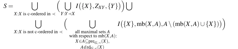
equivalent to the global Markov property for G. For each vertex Vi, ReduceMarkov generates a set of conditional independence relations. If Vi is c-ordered, the relations that correspond to the pairwise Markov property are generated. Otherwise, the relations that correspond to the ordered local Markov property are generated, and Lemma 18 is used to remove some redundant relations. The output S=ReduceMarkov(G,≺)can be described as follows:
S= [
X :X is c-ordered in≺
[
Y :Y≺X
I {X},ZXY,{Y}
[
[
X :X is not c-ordered in≺
[
all maximal sets A with respect to mb(X,A):
X∈A⊆preG,≺(X),
A∈/rdG,≺(X)
I {X},mb(X,A),A\(mb(X,A)∪ {X})
(23)
where ZXY is any set of vertices such that ZXY d-separates X from Y and ∀Z ∈ZXY, d(X,Z)<
d(X,Y).
If a vertex X is c-ordered, O(n) conditional independence relations (or zero partial correla-tions) are added to S. Otherwise, O(2n) conditional independence relations may be added to S and O(n2n)zero partial correlations may be invoked. Furthermore, a c-ordered vertex typically in-volves a smaller conditioning set. I({X},ZXY,{Y})has the conditioning set|ZXY| ≤ |paG(X)|while
I({X},mb(X,A),A\(mb(X,A)∪ {X}))has the conditioning set|mb(X,A)| ≥ |paG(X)|.
Definition 20 (S-Markov Property (S-MP,≺)) Let G be an ADMG and ≺ be a consistent or-dering on the vertices of G. Let S be the set of conditional independence relations given by
ReduceMarkov(G,≺). A probability distribution P is said to satisfy the S-Markov property for G with respect to≺, if
(S-MP,≺) P satisfies all the conditional independence relations in S.
Theorem 21 Let G be an ADMG and ≺ be a consistent ordering on the vertices of G. Let S be the set of conditional independence relations given by ReduceMarkov(G,≺). If a probability distribution P satisfies the composition axiom, then
(GMP)⇐⇒(S-MP,≺).
Proof: (GMP) =⇒ (S-MP,≺) since every conditional independence relation in (S-MP,≺) corre-sponds to a valid d-separation. We show (S-MP,≺) =⇒ (GMP). Without any loss of generality, let≺: V1≺. . .≺Vn. The proof is by induction on the sequence of ordered vertices. Suppose that (S-MP,≺)=⇒(GMP) holds for V1, . . .Vi−1. Let Si−1=I1∪. . .∪Ii−1. Then, by the induction
hypoth-esis, Si−1 contains all the conditional independence relations invoked by (LMP,≺) for V1, . . .Vi−1. If Vi is not c-ordered, Ii=I({Vi},mb(Vi,A),A\(mb(Vi,A)∪ {Vi}))for all maximal ancestral sets
A such that Vi∈A⊆preG,≺(Vi), A∈/ rdG,≺(Vi). The conditional independence relations invoked by (LMP,≺) with respect to Vi and any A∈rdG,≺(Vi) can be derived from other conditional inde-pendence relations by Lemma 18. Thus, Si =Si−1∪Ii contains all the conditional independence relations invoked by (LMP,≺) for V1, . . .Vi, which implies (GMP). If Vi is c-ordered, applying the arguments in the proof of (GMP)⇐⇒(PMP,≺c), we have
I({Vi},paG(Vi),preG,≺(Vi)\({Vi} ∪paG(Vi)∪spG(Vi))).
By the induction hypothesis and the definition of a c-ordered vertex, we have for all Vj∈disG(Vi)∩ preG,≺(Vi)
I({Vj},paG(Vj),preG,≺(Vj)\({Vj} ∪paG(Vj)∪spG(Vj))).
By the arguments in the proof of (GMP)⇐⇒(RLMP,≺c), we have for all maximal ancestral sets A such that Vi∈A⊆preG,≺(Vi)
I({Vi},mb(Vi,A),A\(mb(Vi,A)∪ {Vi})).
V1 V2 V3 V4
W
Figure 8: The c-component{V1,V2,V3,V4}has the root set{V1,V2}
Definition 22 (Root Set) The root set of a c-component C, denoted rt(C)is defined to be the set {Vi∈C|there is no Vj∈C such that a directed path Vj→. . .→Viexists in G}.
For example, the c-component{V1,V2,V3,V4} in Figure 8 has the root set{V1,V2}. V3 and V4 are not in the root set since there are paths V2→V3 and V1→W →V4. The root set has the following properties.
Proposition 23 Let ≺ be a consistent ordering on the vertices of an ADMG G and C be a c-component of G. If the vertices in rt(C) are consecutive in ≺, then all the vertices in rt(C) are c-ordered in≺.
Proof: Assume that the vertices in rt(C) are consecutive in ≺. Then, for X ∈rt(C), disG(X)∩ preG,≺(X)⊆rt(C). Thus, there is no directed edge between any two vertices in disG(X)∩preG,≺(X).
Proposition 24 Let ≺ be a consistent ordering on the vertices of an ADMG G and C be a c-component of G. If a vertex X in C is c-ordered in≺, then X ∈rt(C).
Proof: Assume that X is c-ordered in≺. Suppose for a contradiction that X∈/rt(C). Then, there exists an ancestor Y of X in C. If there exists a vertex Z such that Z∈/C, Y → · · · →Z→ · · · → X . Then, the first condition of a c-ordered vertex is violated. Otherwise, the second condition is
violated.
Proposition 23 and 24 imply that the root set of a component is the largest subset of the c-component that can be c-ordered in a consistent ordering. If G does not have directed mixed cycles, rt(C) =C for every c-component C.
The procedure GetOrdering in Figure 9 is our proposed greedy algorithm that generates a good consistent ordering for G. In Step 1, it searches for the largest root set M and then merges all the vertices in M to one vertex VMmodifying edges accordingly. Then, it repeats the same operation for the modified graph until there is no root set that contains more than one vertex. Since the vertices in a root set are merged at each iteration, the modified graph is acyclic as otherwise there would be a directed path between two vertices in the root set, which contradicts the condition of a root set. After Step 1, we can easily obtain a consistent ordering for the original graph from the modified graph.
4.2 An Example
We show the application of the procedures ReduceMarkov and GetOrdering by considering the ADMG G in Figure 6 (a). First, we apply GetOrdering to get a consistent ordering on the vertices
procedure GetOrdering INPUT: An ADMG G
OUTPUT: A consistent ordering≺on V Step 1:
G0←G (V0is the set of vertices of G)
while (there is a c-component C of G0such that|rt(C)|>1) do
M← /0
for each c-component C of G0do if|rt(C)|>|M|then
M←rt(C) end if end for
Add a vertex VMto GV00\M
Draw an edge VM←X (respectively VM→X , VM↔X ) if there is
Y ←X (respectively Y →X , Y↔X ) in G0such that Y ∈M,X∈V0\M
Let G0be the resulting graph end while
Step 2:
Let≺0 be any consistent ordering on V0. Construct a consistent ordering≺from≺0 by replacing
each VS∈V0\V with the vertices in S (the ordering of the vertices in S is arbitrary)
Figure 9: A greedy algorithm to generate a good consistent ordering on the vertices of an ADMG
G
root set{V6,V7,V8}. Then, the vertices in{V6,V7,V8}are merged into a vertex V678. Figure 6 (b) shows the modified graph G0after the first iteration of the while loop. In the next iteration, we find that every c-component has the root set of size 1. Note that for C={V5,V9}, rt(C) ={V5,V9}in
G but rt(C) ={V5} in G0. Thus, Step 1 ends. In Step 2, from G0 in Figure 6 (b), we can obtain an ordering ≺0: V1 ≺V2≺V3≺V4≺V5≺V678≺V9. This is converted to a consistent ordering
≺: V1≺V2≺V3≺V4≺V5≺V6≺V7≺V8≺V9for G.
With the ordering ≺, we now apply ReduceMarkov to obtain a set of conditional indepen-dence relations that can derive those invoked by the global Markov property. It is easy to see that the vertices V1, . . . ,V8 are c-ordered in≺. Thus, the following conditional independence relations corresponding to the pairwise Markov property are added to the set S (initially empty).
I({V2},/0,{V1}), I({V3},/0,{V2}),
I({V4},/0,{V3,V1}), I({V5},/0,{V4,V3,V2,V1}),
I({V6},/0,{V5,V4,V2}), I({V6},{V3},{V1}),
I({V7},/0,{V5,V4,V2}), I({V7},{V3},{V1}),