Anytime Learning of Decision Trees
Saher Esmeir ESAHER@CS.TECHNION.AC.IL
Shaul Markovitch SHAULM@CS.TECHNION.AC.IL
Department of Computer Science Technion—Israel Institute of Technology Haifa 32000, Israel
Editor: Claude Sammut
Abstract
The majority of existing algorithms for learning decision trees are greedy—a tree is induced top-down, making locally optimal decisions at each node. In most cases, however, the constructed tree is not globally optimal. Even the few non-greedy learners cannot learn good trees when the concept is difficult. Furthermore, they require a fixed amount of time and are not able to generate a better tree if additional time is available. We introduce a framework for anytime induction of decision trees that overcomes these problems by trading computation speed for better tree quality. Our proposed family of algorithms employs a novel strategy for evaluating candidate splits. A biased sampling of the space of consistent trees rooted at an attribute is used to estimate the size of the minimal tree under that attribute, and an attribute with the smallest expected tree is selected. We present two types of anytime induction algorithms: a contract algorithm that determines the sample size on the basis of a pre-given allocation of time, and an interruptible algorithm that starts with a greedy tree and continuously improves subtrees by additional sampling. Experimental results indicate that, for several hard concepts, our proposed approach exhibits good anytime behavior and yields significantly better decision trees when more time is available.
Keywords: anytime algorithms, decision tree induction, lookahead, hard concepts, resource-bounded reasoning
1. Introduction
Assume that a medical center has decided to use medical records of previous patients in order to build an automatic diagnostic system for a particular disease. The center applies the C4.5 algorithm on thousands of records, and after few seconds receives a decision tree. During the coming months, or even years, the same induced decision tree will be used to predict whether patients have or do not have the disease. Obviously, the medical center is willing to wait much longer to obtain a better tree—either more accurate or more comprehensible.
Consider also a planning agent that has to learn a decision tree from a given set of examples, while the time at which the model will be needed by the agent is not known in advance. In this case, the agent would like the learning procedure to learn the best tree it can until it is interrupted and queried for a solution.
a1 a2 a3 a4 label
1 0 0 1 +
0 1 0 0 +
0 0 0 0
-1 1 0 0
-0 1 1 1 +
0 0 1 1
-1 0 1 1 +
(a) A set of training instances.
- +
+
- +
-(b) ID3’s performance.
Figure 1: Learning the 2-XOR concept a1⊕a2, where a3and a4are irrelevant
applications such as game playing, planning, stock trading and e-mail filtering. In this work, we introduce a framework for exploiting extra time, preallocated or not, in order to learn better models. Despite the recent progress in advanced induction algorithms such as SVM (Vapnik, 1995), decision trees are still considered attractive for many real-life applications, mostly due to their interpretability (Hastie et al., 2001, chap. 9). Craven (1996) lists several reasons why the under-standability of a model by humans is an important criterion for evaluating it. These reasons include, among others, the possibility for human validation of the model and generation of human-readable explanations for the classifier predictions. When classification cost is important, decision trees may be attractive in that they ask only for the values of the features along a single path from the root to a leaf. In terms of accuracy, decision trees have been shown to be competitive with other classifiers for several learning tasks.
The majority of existing methods for decision tree induction build a tree top-down and use local measures in an attempt to produce small trees, which, by Occam’s Razor (Blumer et al., 1987), should have better predictive power. The well-known C4.5 algorithm (Quinlan, 1993) uses the gain ratio as a heuristic for predicting which attribute will yield a smaller tree. Several other alternative local greedy measures have been developed, among which are ID3’s information gain, Gini index (Breiman et al., 1984), and chi-square (Mingers, 1989). Mingers (1989) reports an empirical comparison of several measures, and concludes that the predictive accuracy of the induced trees is not sensitive to the choice of split measure and even random splits do not significantly decrease accuracy. Buntine and Niblett (1992) present additional results on further domains and conclude that while random splitting leads to inferior trees, the information gain and Gini index measures are statistically indistinguishable.
The top-down methodology has the advantage of evaluating a potential attribute for a split in the context of the attributes associated with the nodes above it. The local greedy measures, how-ever, consider each of the remaining attributes independently, ignoring potential interaction between different attributes (Mingers, 1989; Kononenko et al., 1997; Kim and Loh, 2001). We refer to the family of learning tasks where the utility of a set of attributes cannot be recognized by examining only subsets of it as tasks with a strong interdependency. When learning a problem with a strong interdependency, greedy measures can lead to a choice of non-optimal splits. To illustrate the above,
As-sume that the set of examples is as listed in Figure 1(a). We observe that gain-1 of the irrelevant
attribute a4is the highest:
0.13=gain1(a4)>gain1(a1) =gain1(a2) =gain1(a3) =0.02,
and hence ID3 would choose attribute a4 first. Figure 1(b) gives the decision tree as produced by
ID3. Any positive instance with value 0 for a4 would be misclassified by this decision tree. In the
general case of parity concepts, the information gain measure is unable to distinguish between the relevant and irrelevant attributes because neither has a positive gain. Consequently, the learner will grow an overcomplicated tree with splits on irrelevant variables that come either in addition to or instead of the desired splits.
The problem of finding the smallest consistent tree1 is known to be NP-complete (Hyafil and
Rivest, 1976; Murphy and McCraw, 1991). In many applications that deal with hard problems, we are ready to allocate many more resources than required by simple greedy algorithms, but still cannot afford algorithms of exponential complexity. One commonly proposed approach for hard problems is anytime algorithms (Boddy and Dean, 1994), which can trade computation speed for quality. Quinlan (1993, chap. 11) recognized the need for this type of anytime algorithm for decision tree learning: “What is wanted is a resource constrained algorithm that will do the best it can within a specified computational budget and can pick up threads and continue if this budget is increased. This would make a challenging thesis topic!”
There are two main classes of anytime algorithms, namely contract and interruptible (Russell and Zilberstein, 1996). A contract algorithm is one that gets its resource allocation as a parameter. If interrupted at any point before the allocation is completed, it might not yield any useful results. An interruptible algorithm is one whose resource allocation is not given in advance and thus must be prepared to be interrupted at any moment. While the assumption of preallocated resources holds for many induction tasks, in many other real-life applications it is not possible to allocate the resources in advance. Therefore, in our work, we are interested both in contract and interruptible decision tree learners.
In this research, we suggest exploiting additional time resources by performing lookahead. Lookahead search is a well-known technique for improving greedy algorithms (Sarkar et al., 1994). When applied to decision tree induction, lookahead attempts to predict the profitability of a split at a node by estimating its effect on deeper descendants of the node. One of the main disadvantages of the greedy top-down strategy is that the effect of a wrong split decision is propagated down to all the nodes below it (Hastie et al., 2001, chap. 9). Lookahead search attempts to predict and avoid such non-contributive splits during the process of induction, before the final decision at each node is made.
Lookahead techniques have been applied to decision tree induction by several researchers. The reported results vary from lookahead produces better trees (Norton, 1989; Ragavan and Rendell, 1993; Dong and Kothari, 2001) to lookahead does not help and can hurt (Murthy and Salzberg, 1995). One problem with these works is their use of a uniform, fixed low-depth lookahead, therefore disqualifying the proposed algorithms from serving as anytime algorithms. Another problem is the data sets on which the lookahead methods were evaluated. For simple learning tasks, such as induction of conjunctive concepts, greedy methods perform quite well and no lookahead is needed. However, for more difficult concepts such as XOR, the greedy approach is likely to fail. Few other
Procedure TDIDT(E,A) If E=/0Return Leaf(nil)
If∃c such that∀e∈E Class(e) =c
Return Leaf(c)
a←CHOOSE-ATTRIBUTE(A,E)
V ←domain(a)
Foreach vi∈V
Ei← {e∈E|a(e) =vi}
Si←TDIDT(Ei,A− {a})
Return Node(a,{hvi,Sii |i=1. . .|V|})
Figure 2: Procedure for top-down induction of decision trees. E stands for the set of examples and A stands for the set of attributes.
non-greedy decision tree learners have been recently introduced (Bennett, 1994; Utgoff et al., 1997; Papagelis and Kalles, 2001; Page and Ray, 2003). These works, however, are not capable to handle
high-dimensional difficult concepts and are not designed to offer anytime behavior.2 The main
challenge we face in this work is to make use of extra resources to induce better trees for hard concepts. Note that in contrast to incremental induction (Utgoff, 1989), we restrict ourselves in this paper to batch setup where all the training instances are available beforehand.
2. Contract Anytime Induction of Decision Trees
TDIDT (top-down induction of decision trees) methods start from the entire set of training examples, partition it into subsets by testing the value of an attribute, and then recursively call the induction algorithm for each subset. Figure 2 formalizes the basic algorithm for TDIDT. We focus first on consistent trees for which the stopping criterion for the top-down recursion is when all the examples have the same class label. Later, we consider pruning, which allows simpler trees at the cost of possible inconsistency with the training data (Breiman et al., 1984; Quinlan, 1993).
In this work we propose investing more time resources for making better split decisions. We first discuss tree size as a desired property of the tree to be learned and then we describe an anytime algorithm that uses sampling methods to obtain smaller trees.
2.1 Inductive Bias in Decision Tree Induction
The hypothesis space of TDIDT is huge and a major question is what strategy should be followed to direct the search. In other words, we need to decide what our preference bias (Mitchell, 1997,
chap. 3) will be. This preference bias will be expressed in the CHOOSE-ATTRIBUTEprocedure that
determines which tree is explored next.
Ultimately, we would like to follow a policy that maximizes the accuracy of the tree on unseen examples. However, since these examples are not available, a heuristic should be used. Motivated by Occam’s Razor, a widely adopted approach is to prefer smaller trees. The utility of this principle
to machine learning algorithms has been the subject of a heated debate. Several studies attempted to justify Occam’s razor with theoretical and empirical arguments (Blumer et al., 1987; Quinlan and Rivest, 1989; Fayyad and Irani, 1990). But a number of recent works have questioned the utility of Occam’s razor, and provided theoretical and experimental evidence against it.
Quinlan and Cameron-Jones (1995) provided empirical evidence that oversearching might result in less accurate rules. Experimental results with several UCI data sets indicate that the complexity of the produced theories does not correlate well with their accuracy, a finding that is inconsistent with Occam’s Razor. Schaffer (1994) proved that no learning bias can outperform another bias over the space of all possible learning tasks. This looks like theoretical evidence against Occam’s razor. Rao et al. (1995), however, argued against the applicability of this result to real-world problems by questioning the validity of its basic assumption about the uniform distribution of possible learning tasks. Webb (1996) presented C4.5X, an extension to C4.5 that uses similarity considerations to further specialize consistent leaves. Webb reported an empirical evaluation which shows that C4.5X has a slight advantage in a few domains and argued that these results discredit Occam’s thesis.
Murphy and Pazzani (1994) reported a set of experiments in which all the possible consistent decision trees were produced and showed that, for several tasks, the smallest consistent decision tree had higher predictive error than slightly larger trees. However, when the authors compared the likelihood of better generalization for smaller vs. more complex trees, they concluded that simpler hypotheses should be preferred when no further knowledge of the target concept is available. The small number of training examples relative to the size of the tree that perfectly describes the concept might explain why, in these cases, the smallest tree did not generalize best. Another reason could be that only small spaces of decision trees were explored. To verify these explanations, we use a similar experimental setup where the data sets have larger training sets and attribute vectors of higher dimensionality. Because the number of all possible consistent trees is huge, we use a Random Tree Generator (RTG) to sample the space of trees obtainable by TDIDT algorithms. RTG builds a tree top-down and chooses the splitting attribute at random.
We report the results for three data sets: XOR-5, Tic-tac-toe, and Zoo (See Appendix A for detailed descriptions of these data sets). For each data set, the examples were partitioned into a training set (90%) and a testing set (10%), and RTG was used to generate a sample of 10 million consistent decision trees. The behavior in the three data sets is similar: the accuracy monotonically decreases with the increase in the size of the trees (number of leaves), confirming the utility of Occam’s Razor. Further experiments with a variety of data sets indicate that the inverse correlation between size and accuracy is statistically significant (Esmeir and Markovitch, 2007).
It is important to note that smaller trees have several advantages aside from their probable greater accuracy, such as greater statistical evidence at the leaves, better comprehensibility, lower storage costs, and faster classification (in terms of total attribute evaluations).
Motivated by the above discussion, our goal is to find the smallest consistent tree. In TDIDT, the learner has to choose a split at each node, given a set of examples E that reach the node and a
set of unused attributes A. For each attribute a, let Tmin(a,A,E)be the smallest tree rooted at a that
is consistent with E and uses attributes from A− {a}for the internal splits. Given two candidate
attributes a1 and a2, we obviously prefer the attribute whose associated Tmin(a)is the smaller. For
a set of attributes A, we defineA to be the set of attributes whose associated Te min(a)is the smaller.
Formally,Ae=arg mina∈ATmin(a). We say that a splitting attribute a is optimal if a∈A. Observee
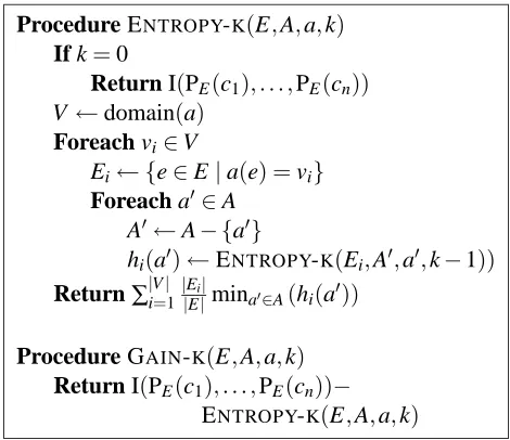
Procedure ENTROPY-K(E,A,a,k)
If k=0
Return I(PE(c1), . . . ,PE(cn))
V ←domain(a)
Foreach vi∈V
Ei← {e∈E|a(e) =vi}
Foreach a0∈A
A0←A− {a0}
hi(a0)←ENTROPY-K(Ei,A0,a0,k−1))
Return∑|iV=|1||EEi||mina0∈A(hi(a0)) Procedure GAIN-K(E,A,a,k)
Return I(PE(c1), . . . ,PE(cn))−
ENTROPY-K(E,A,a,k)
Figure 3: Procedures for computing entropykand gaink for attribute a
2.2 Fixed-depth Lookahead
One possible approach for improving greedy TDIDT algorithms is to lookahead in order to examine the effect of a split deeper in the tree. ID3 uses entropy to test the effect of using an attribute one level below the current node. This can be extended to allow measuring the entropy at any depth k below the current node. This approach was the basis for the IDX algorithm (Norton, 1989). The
recursive definition minimizes the k−1 entropy for each child and computes their weighted average.
Figure 3 describes an algorithm for computing entropykand its associated gaink. Note that the gain
computed by ID3 is equivalent to gaink for k=1. We refer to this lookahead-based variation of ID3
as ID3-k. At each tree node, ID3-k chooses the attribute that maximizes gaink.3
ID3-k can be viewed as a contract anytime algorithm parameterized by k. However, despite its ability to exploit additional resources when available, the anytime behavior of ID3-k is problematic.
The run time of ID3-k grows exponentially as k increases.4 As a result, the gap between the points
of time at which the resulting tree can improve grows wider, limiting the algorithm’s flexibility. Furthermore, it is quite possible that looking ahead to depth k will not be sufficient to find an
op-timal split. Entropyk measures the weighted average of the entropy in depth k but does not give a
direct estimation of the resulting tree size. Thus, when k<|A|, this heuristic is more informed than
entropy1 but can still produce misleading results. In most cases we do not know in advance what
value of k would be sufficient for correctly learning the target concept. Invoking exhaustive
looka-head, that is, lookahead to depth k=|A|, will obviously lead to optimal splits, but its computational
costs are prohibitively high. In the following subsection, we propose an alternative approach for evaluating attributes that overcomes the above-mentioned drawbacks of ID3-k.
3. If two attributes yield the same decrease in entropy, we prefer the one whose associated lookahead tree is shallower. 4. For example, in the binary case, ID3-k explores∏ki=−01(n−i)2i
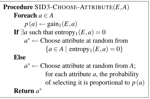
Procedure SID3-CHOOSE-ATTRIBUTE(E,A)
Foreach a∈A
p(a)←gain1(E,a)
If∃a such that entropy1(E,a) =0
a∗←Choose attribute at random from
{a∈A|entropy1(E,a) =0}
Else
a∗←Choose attribute at random from A;
for each attribute a, the probability
of selecting it is proportional to p(a)
Return a∗
Figure 4: Attribute selection in SID3
2.3 Estimating Tree Size by Sampling
Motivated by the advantages of smaller decision trees, we introduce a novel algorithm that, given an attribute a, evaluates it by estimating the size of the minimal tree under it. The estimation is based on Monte-Carlo sampling of the space of consistent trees rooted at a. We estimate the minimum by the size of the smallest tree in the sample. The number of trees in the sample depends on the available resources, where the quality of the estimation is expected to improve with the increased sample size.
One way to sample the space of trees is to repeatedly produce random consistent trees using the RTG procedure. Since the space of consistent decision trees is large, such a sample might be a poor representative and the resulting estimation inaccurate. We propose an alternative sampling approach that produces trees of smaller expected size. Such a sample is likely to lead to a better estimation of the minimum.
Our approach is based on a new tree generation algorithm that we designed, called Stochastic ID3 (SID3). Using this algorithm repeatedly allows the space of “good” trees to be sampled semi-randomly. In SID3, rather than choose an attribute that maximizes the information gain, we choose the splitting attribute randomly. The likelihood that an attribute will be chosen is proportional to
its information gain.5 However, if there are attributes that decrease the entropy to zero, then one of
them is picked randomly. The attribute selection procedure of SID3 is listed in Figure 4.
To show that SID3 is a better sampler than RTG, we repeated our sampling experiment (Section 2.1) using SID3 as the sample generator. Figure 5 compares the frequency curves of RTG and SID3. Relative to RTG, the graph for SID3 is shifted to the left, indicating that the SID3 trees are clearly smaller. Next, we compared the average minimum found for samples of different sizes. Figure 6 shows the results. For the three data sets, the minimal size found by SID3 is strictly smaller than the value found by RTG. Given the same budget of time, RTG produced, on average, samples that are twice as large as that of SID3. However, even when the results are normalized (dashed line), SID3 is still superior.
Having decided about the sampler, we are ready to describe our proposed contract algorithm, Lookahead-by-Stochastic-ID3 (LSID3). In LSID3, each candidate split is evaluated by the estimated
0 0.05 0.1 0.15 0.2 0.25 0.3
40 60 80 100 120 140 160 180
Frequency
Size RTG
SID3
0 0.02 0.04 0.06 0.08 0.1 0.12 0.14 0.16 0.18 0.2
150 200 250 300 350 400 450 500 550 600
Frequency
Size RTG
SID3
0 0.05 0.1 0.15 0.2 0.25 0.3 0.35
15 20 25 30 35 40 45 50 55
Frequency
Size RTG SID3
Figure 5: Frequency curves for the XOR-5 (left), Tic-tac-toe, and Zoo (right) data sets
80 90 100 110 120 130 140
0 5 10 15 20 25 30
Minimum
Size SID3 N-SID3 RTG
250 300 350 400 450 500
0 5 10 15 20 25 30
Minimum
Size SID3 N-SID3 RTG
10 12 14 16 18 20 22 24
0 5 10 15 20 25 30
Minimum
Size SID3 N-SID3 RTG
Figure 6: The minimum as estimated by SID3 and RTG as a function of the sample size. The data sets are XOR5 (left), Tic-tac-toe and Zoo (right). The dashed line describes the results for SID3 normalized by time.
size of the subtree under it. To estimate the size under an attribute a, LSID3 partitions the set of examples according to the values a can take and repeatedly invokes SID3 to sample the space of trees consistent with each subset. Summing up the minimal tree size for each subset gives an estimation of the minimal total tree size under a.
LSID3 is a contract algorithm parameterized by r, the sample size. LSID3 with r=0 is defined
to choose the splitting attribute using the standard ID3 selection method. Figure 7 illustrates the choice of splitting attributes as made by LSID3. In the given example, SID3 is called twice for each
subset and the evaluation of the examined attribute a is the sum of the two minima: min(4,3) +
min(2,6) =5. The method for choosing a splitting attribute is formalized in Figure 8.
To analyze the time complexity of LSID3, let m be the total number of examples and n be the
total number of attributes. For a given node y, we denote by nythe number of candidate attributes
at y, and by my the number of examples that reach y. ID3, at each node y, calculates gain for ny
attributes using myexamples, that is, the complexity of choosing an attribute is O(ny·my). At level i
of the tree, the total number of examples is bounded by m and the number of attributes to consider is
n−i. Thus, it takes O(m·(n−i))to find the splits for all nodes in level i. In the worst case the tree
will be of depth n and hence the total runtime complexity of ID3 will be O(m·n2)(Utgoff, 1989).
Shavlik et al. (1991) reported for ID3 an empirically based average-case complexity of O(m·n).
Figure 7: Attribute evaluation using LSID3. The estimated subtree size for a is min(4,3) +
min(2,6) =5.
Procedure LSID3-CHOOSE-ATTRIBUTE(E,A,r)
If r=0
Return ID3-CHOOSE-ATTRIBUTE(E, A) Foreach a∈A
Foreach vi∈domain(a)
Ei← {e∈E|a(e) =vi}
mini←∞
Repeat r times
mini←min(mini,|SID3(Ei,A− {a})|)
totala←∑|idomain=1 (a)|mini
Return a for which totalais minimal
Figure 8: Attribute selection in LSID3
write the complexity of LSID3(r) as
n−1
∑
i=0
r·(n−i)·O(m·(n−i)2) =
n
∑
i=1
O(r·m·i3) =O(r·m·n4).
In the average case, we replace the runtime of SID3 by O(m·(n−i)), and hence we have
n−1
∑
i=0
r·(n−i)·O(m·(n−i)) =
n
∑
i=1
O(r·m·i2) =O(r·m·n3). (1)
According to the above analysis, the run-time of LSID3 grows at most linearly with r (under the assumption that increasing r does not result in larger trees). We expect that increasing r will improve the classifier’s quality. To understand why, let us examine the expected behavior of the
LSID3 algorithm on the 2-XOR problem used in Figure 1(b). LSID3 with r=0, which is equivalent
calling SID3 to estimate the size of the trees rooted at a. The attribute with the smallest estimation
will be selected. The minimal size for trees rooted at a4 is 6 and for trees rooted at a3 is 7. For
a1 and a2, SID3 would necessarily produce trees of size 4.6 Thus, LSID3, even with r=1, will
succeed in learning the right tree. For more complicated problems such as 3-XOR, the space of SID3 trees under the relevant attributes includes trees other than the smallest. In that case, the larger the sample is, the higher the likelihood is that the smallest tree will be drawn.
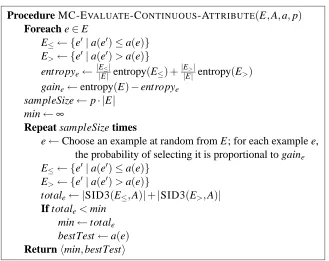
2.4 Evaluating Continuous Attributes by Sampling the Candidate Cuts
When attributes have a continuous domain, the decision tree learner needs to discretize their values in order to define splitting tests. One common approach is to partition the range of values an attribute can take into bins, prior to the process of induction. Dougherty et al. (1995) review and compare several different strategies for pre-discretization. Using such a strategy, our lookahead algorithm can operate unchanged. Pre-discretization, however, may be harmful in many domains because the correct partitioning may differ from one context (node) to another.
An alternative approach is to determine dynamically at each node a threshold that splits the
examples into two subsets. The number of different possible thresholds is at most |E| −1, and
thus the number of candidate tests to consider for each continuous attribute increases to O(|E|).
Such an increase in complexity may be insignificant for greedy algorithms, where evaluating each split requires a cheap computation (like information gain in ID3). In LSID3, however, the dynamic method may present a significant problem because evaluating the usefulness of each candidate split is very costly.
The desired method would reduce the number of splits to evaluate while avoiding the disadvan-tages of pre-discretization. We devised a method for controlling the resources devoted to evaluating a continuous attribute by Monte Carlo sampling of the space of splits. Initially, we evaluate each
possible splitting test by the information gain it yields. This can be done in linear time O(|E|).
Next, we choose a sample of the candidate splitting tests where the probability that a test will be chosen is proportional to its information gain. Each candidate in the sample is evaluated by a single invocation of SID3. However, since we sample with repetitions, candidates with high information gain may have multiple instances in the sample, resulting in several SID3 invocations.
The resources allocated for evaluating a continuous attribute using the above method are deter-mined by the sample size. If our goal is to devote a similar amount of resources to all attributes, then we can use r as the size of the sample. Such an approach, however, does not take into account the size of the population to be sampled. We use a simple alternative approach of taking samples
with size p· |E|where p is a predetermined parameter, set by the user according to the available
resources.7 Note that p can be greater than one because we sample with repetition.
We name this variant of the LSID3 algorithm MC, and formalize it in Figure 9. LSID3-MC can serve as an anytime algorithm that is parameterized by p and r.
2.5 Multiway vs. Binary Splits
The TDIDT procedure, as described in Figure 2, partitions the current set of examples into subsets according to the different values the splitting attribute can take. LSID3, which is a TDIDT algo-rithm, inherits this property. While multiway splits can yield more comprehensible trees (Kim and
6. Neither a3nor a4can be selected at the 2ndlevel since the remaining relevant attribute reduces the entropy to zero.
Procedure MC-EVALUATE-CONTINUOUS-ATTRIBUTE(E,A,a,p)
Foreach e∈E
E≤← {e0|a(e0)≤a(e)}
E>← {e0|a(e0)>a(e)}
entropye← |E|E≤||entropy(E≤) +|E|E>||entropy(E>)
gaine←entropy(E)−entropye
sampleSize←p· |E|
min←∞
Repeat sampleSize times
e←Choose an example at random from E; for each example e,
the probability of selecting it is proportional to gaine
E≤← {e0|a(e0)≤a(e)}
E>← {e0|a(e0)>a(e)}
totale← |SID3(E≤,A)|+|SID3(E>,A)|
If totale<min
min←totale
bestTest←a(e)
Returnhmin,bestTesti
Figure 9: Monte Carlo evaluation of continuous attributes using SID3
Loh, 2001), they might fragment the data too quickly, decreasing its learnability (Hastie et al., 2001, chap. 9).
To avoid the fragmentation problem, several learners take a different approach and consider only binary splits (e.g., CART and QUEST, Loh and Shih, 1997). One way to obtain binary splits when an attribute a is categorical is to partition the examples using a single value v: all the examples
with a=v are bagged into one group and all the other examples are bagged into a second group.
Therefore, for each attribute a there are|domain(a)|candidate splits. While efficient, this strategy
does not allow different values to be combined, and therefore might over-fragment the data. CART
overcomes this by searching over all non-empty subsets of domain(a). We denote by BLSID3 a
variant of LSID3 that yields binary trees and adopts the CART style exhaustive search. Observe
that the complexity of evaluating an attribute in BLSID3 is O(2|domain(a)|)times that in LSID3.
A second problem with LSID3’s multiway splits is their bias in attribute selection. Consider
for example a learning task with four attributes: three binary attributes a1,a2,a3, and a categorical
attribute a4whose domain is{A,C,G,T}. Assume that the concept is a1⊕a2and that a4was created
from the values of a2by randomly and uniformly mapping every 0 into A or C and every 1 into G
or T . Theoretically, a2and a4are equally important to the class. LSID3, however, would prefer to
split a2due to its smaller associated total tree size.8 BLSID3 solves this problem by considering the
binary test∈ {A,C}.
Loh and Shih (1997) pointed out that exhaustive search tends to prefer features with larger domains and proposed QUEST, which overcomes this problem by dealing with attribute selection and with test selection separately: first an attribute is chosen and only then is the best test picked.
!"$#%& %'$(
#
'
)+*,
- )+*.,
/
0
1
0
/
234
5
678 9:
9;
- )+*.,<
Figure 10: The space of decision trees over a set of attributes A and a set of examples E
This bias, and its reduction by QUEST, were studied in the context of greedy attribute evaluation, but can potentially be applied to our non-greedy approach.
2.6 Pruning the LSID3 Trees
Pruning tackles the problem of how to avoid overfitting the data, mainly in the presence of classifi-cation noise. It is not designed, however, to recover from wrong greedy decisions. When there are sufficient examples, wrong splits do not significantly diminish accuracy, but result in less compre-hensible trees and costlier classification. When there are fewer examples the problem is intensified because the accuracy is adversely affected. In our proposed anytime approach, this problem is tack-led by allotting additional time for reaching trees unexplored by greedy algorithms with pruning. Therefore, we view pruning as orthogonal to lookahead and suggest considering it as an additional phase in order to avoid overfitting.
Pruning can be applied in two different ways. First, it can be applied as a second phase after each LSID3 final tree has been built. We denote this extension by LSID3-p (and BLSID3-p for binary splits). Second, it is worthwhile to examine pruning of the lookahead trees. For this purpose, a post-pruning phase will be applied to the trees that were generated by SID3 to form the lookahead sample, and the size of the pruned trees will be considered. The expected contribution of pruning in this case is questionable since it has a similar effect on the entire lookahead sample.
Previous comparative studies did not find a single pruning method that is generally the best and conclude that different pruning techniques behave similarly (Esposito et al., 1997; Oates and Jensen, 1997). Therefore, in our experiments we adopt the same pruning method as in C4.5, namely error-based pruning (EPB), and examine post-pruning of the final trees as well as pruning of the lookahead trees.
Figure 10 describes the spaces of decision trees obtainable by LSID3. Let A be a set of attributes and E be a set of examples. The space of decision trees over A can be partitioned into two: the space of trees consistent with E and the space of trees inconsistent with E. The space of consistent trees
includes as a subspace the trees inducible by TDIDT.9The trees that ID3 can produce are a subspace
of the TDIDT space. Pruning extends the space of ID3 trees to the inconsistent space. LSID3
can reach trees that are obtainable by TDIDT but not by the greedy methods and their extensions. LSID3-p expands the search space to trees that do not fit the training data perfectly, so that noisy training sets can be handled.
2.7 Mapping Contract Time to Sample Size
LSID3 is parameterized by r, the number of times SID3 is invoked for each candidate. In real-life applications, however, the user supplies the system with the time she is willing to allocate for the learning process. Hence, a mapping from the contract time to r is needed.
One way to obtain such a mapping is to run the algorithm with r=1. Since the runtime grows
linearly with r, one can now, given the remaining time and the runtime for r=1, easily find the
corresponding value of r. Then, the whole induction process is restarted with the measured r as the contract parameter. The problem with this method is that, in many cases, running the algorithm
with r=1 consumes many of the available resources while not contributing to the final classifier.
Another possibility is mapping time to r on the basis of previous experience on the same domain or a domain with similar properties. When no such knowledge exists, one can derive the runtime from the time complexity analysis. However, in practice, the runtime is highly dependent on the complexity of the domain and the number of splits that in fact take place. Hence it is very difficult to predict.
3. Interruptible Anytime Learning of Decision Trees
As a contract algorithm, LSID3 assumes that the contract parameter is known in advance. In many real-life cases, however, either the contract time is unknown or mapping the available resources to the appropriate contract parameter is not possible. To handle such cases, we need to devise an interruptible anytime algorithm.
We start with a method that converts LSID3 to an interruptible algorithm using the general sequencing technique described by Russell and Zilberstein (1996). This conversion, however, uses the contract algorithm as a black box and hence cannot take into account specific aspects of decision tree induction. Next, we present a novel iterative improvement algorithm, Interruptible Induction of Decision Trees (IIDT), that repeatedly replaces subtrees of the current hypothesis with subtrees generated with higher resource allocation and thus expected to be better.
3.1 Interruptible Induction by Sequencing Contract Algorithms
By definition, every interruptible algorithm can serve as a contract algorithm because one can stop the interruptible algorithm when all the resources have been consumed. Russell and Zilberstein
(1996) showed that the other direction works as well: any contract algorithm
A
can be convertedinto an interruptible algorithm
B
with a constant penalty.B
is constructed by runningA
repeatedlywith exponentially increasing time limits. This general approach can be used to convert LSID3 into
an interruptible algorithm. LSID3 gets its contract time in terms of r, the sample size. When r=0,
LSID3 is defined to be identical to ID3. Therefore, we first call LSID3 with r=0 and then continue
with exponentially increasing values of r, starting from r=1. Figure 11 formalizes the resulting
Procedure SEQUENCED-LSID3(E,A)
T ←ID3(E,A)
r←1
While not-interrupted
T ←LSID3(E,A,r)
r←2·r
Return T
Figure 11: Conversion of LSID3 to an interruptible algorithm by sequenced invocations
One problem with the sequencing approach is the exponential growth of the gaps between the times at which an improved result can be obtained. The reason for this problem is the generality of the sequencing approach, which views the contract algorithm as a black box. Thus, in the case of LSID3, at each iteration the whole decision tree is rebuilt. In addition, the minimal value that can
be used forτ is the runtime of LSID3(r=1). In many cases we would like to stop the algorithm
earlier. When we do, the sequencing approach will return the initial greedy tree. Our interruptible anytime framework, called IIDT, overcomes these problems by iteratively improving the tree rather than trying to rebuild it.
3.2 Interruptible Induction by Iterative Improvement
Iterative improvement approaches that start with an initial solution and repeatedly modify it have been successfully applied to many AI domains, such as CSP, timetabling, and combinatorial prob-lems (Minton et al., 1992; Johnson et al., 1991; Schaerf, 1996). The key idea behind iterative improvement techniques is to choose an element of the current suboptimal solution and improve it by local repairs. IIDT adopts the above approach for decision tree learning and iteratively re-vises subtrees. It can serve as an interruptible anytime algorithm because, when interrupted, it can immediately return the currently best solution available.
As in LSID3, IIDT exploits additional resources in an attempt to produce better decision trees. The principal difference between the algorithms is that LSID3 uses the available resources to in-duce a decision tree top-down, where each decision made at a node is final and does not change. IIDT, however, is not allocated resources in advance and uses extra time resources to modify split decisions repeatedly.
IIDT receives a set of examples and a set of attributes. It first performs a quick construction of an initial decision tree by calling ID3. Then it iteratively attempts to improve the current tree by choosing a node and rebuilding its subtree with more resources than those used previously. If the newly induced subtree is better, it will replace the existing one. IIDT is formalized in Figure 12.
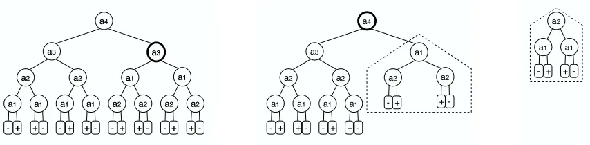
Figure 13 illustrates how IIDT works. The target concept is a1⊕a2, with two additional
irrel-evant attributes, a3 and a4. The leftmost tree was constructed using ID3. In the first iteration, the
Procedure IIDT(E,A)
T ←ID3(E,A)
While not-interrupted
node←CHOOSE-NODE(T,E,A)
t← subtree of T rooted at node
Anode← {a∈A|a∈/ ancestor of node}
Enode← {e∈E|e reaches node}
r←NEXT-R(node)
t0←REBUILD-TREE(Enode,Anode,r)
If EVALUATE(t)>EVALUATE(t0)
replace t with t0
Return T
Figure 12: Interruptible induction of decision trees
a4
a3
a2
a1 a1
a2
a1 a1
a1
a2 a2
- + + - - + +
-+
+
-a2
a1 a1
- + +
-Figure 13: Iterative improvement of the decision tree produced for the 2-XOR concept a1⊕a2
with two additional irrelevant attributes, a3 and a4. The leftmost tree was constructed
using ID3. In the first iteration the subtree rooted at the bolded node is selected for improvement and replaced by a smaller tree (surrounded by a dashed line). Next, the root is selected for improvement and the whole tree is replaced by a tree that perfectly describes the concept.
IIDT is designed as a general framework for interruptible learning of decision trees. It can use different approaches for choosing which node to improve, for allocating resources for an improve-ment iteration, for rebuilding a subtree, and for deciding whether an alternative subtree is better.
3.2.1 CHOOSING ASUBTREE TOIMPROVE
Intuitively, the next node we would like to improve is the one with the highest expected marginal utility, that is, the one with the highest ratio between the expected benefit and the expected cost (Hovitz, 1990; Russell and Wefald, 1989). Estimating the expected gain and expected cost of re-building a subtree is a difficult problem. There is no apparent way to estimate the expected im-provement in terms of either tree size or generalization accuracy. In addition, the resources to be consumed by LSID3 are difficult to predict precisely. We now show how to approximate these values, and how to incorporate these approximations into the node selection procedure.
Resource Allocation. The LSID3 algorithm receives its resource allocation in terms of r, the number of samplings devoted to each attribute. Given a tree node y, we can view the task of re-building the subtree below y as an independent task. Every time y is selected, we have to allocate resources for the reconstruction process. Following Russell and Zilberstein (1996), the optimal strategy in this case is to double the amount of resources at each iteration. Thus, if the resources
allocated for the last attempted improvement of y were LAST-R(y), the next allocation will be
NEXT-R(y) =2·LAST-R(y).
Expected Cost. The expected cost can be approximated using the average time complexity of the
contract algorithm used to rebuild subtrees. Following Equation 1, we estimate NEXT-R(y)·m·n3to
be the expected runtime of LSID3 when rebuilding a node y, where m is the number of examples that reach y and n is the number of attributes to consider. We observe that subtrees rooted in deeper levels are preferred because they have fewer examples and attributes to consider. Thus, their expected runtime is shorter. Furthermore, because each time allocation for a node doubles the previous one, nodes that have already been selected many times for improvement will have higher associated costs and are less likely to be chosen again.
Expected benefit. The whole framework of decision tree induction rests on the assumption that smaller consistent trees are better than larger ones. Therefore, the size of a subtree can serve as a measure for its quality. It is difficult, however, to estimate the size of the reconstructed subtree without actually building it. Therefore, we use instead an upper limit on the possible reduction in size. The minimal size possible for a decision tree is obtained when all examples are labelled with the same class. Such cases are easily recognized by the greedy ID3. Similarly, if a subtree were replaceable by another subtree of depth 1, ID3 (and LSID3) would have chosen the smaller subtree. Thus, the maximal reduction of the size of an existing subtree is to the size of a tree of depth 2. Assuming that the maximal number of values per attribute is b, the maximal size of such a tree is
b2. Hence, an upper bound on the benefit from reconstructing an existing tree t is SIZE(t)−b2.
Ignoring the expected costs and considering only the expected benefits results in giving the highest score to the root node. This makes sense: assuming that we have infinite resources, we would attempt to improve the entire tree rather than parts of it.
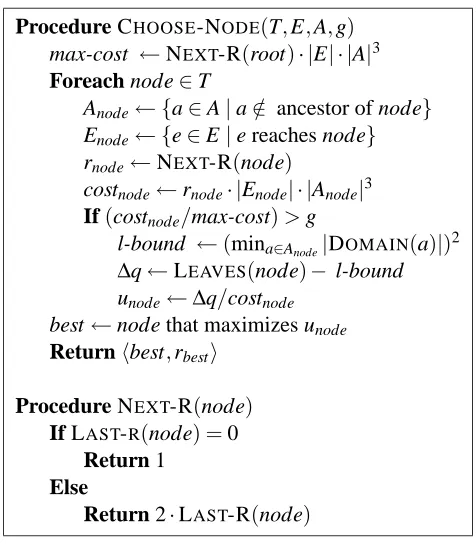
Procedure CHOOSE-NODE(T,E,A,g)
max-cost ←NEXT-R(root)· |E| · |A|3
Foreach node∈T
Anode← {a∈A|a∈/ ancestor of node}
Enode← {e∈E|e reaches node}
rnode←NEXT-R(node)
costnode←rnode· |Enode| · |Anode|3
If(costnode/max-cost)>g
l-bound ←(mina∈Anode|DOMAIN(a)|)
2
∆q←LEAVES(node)− l-bound
unode←∆q/costnode
best←node that maximizes unode
Returnhbest,rbesti
Procedure NEXT-R(node) If LAST-R(node) =0
Return 1 Else
Return 2·LAST-R(node)
Figure 14: Choosing a node for reconstruction
nodes will have been wasted. Had the algorithm first selected the upper level trees, this waste would have been avoided, but the time gaps between potential improvements would have increased.
To control the tradeoff between efficient resource use and anytime performance flexibility, we
add a granularity parameter 0≤g≤1. This parameter serves as a threshold for the minimal time
allocation for an improvement phase. A node can be selected for improvement only if its normalized expected cost is above g. To compute the normalized expected cost, we divide the expected cost by the expected cost of the root node. Note that it is possible to have nodes with a cost that is higher than the cost of the root node, since the expected cost doubles the cost of the last improvement of the node. Therefore, the normalized expected cost can be higher than 1. Such nodes, however, will never be selected for improvement, because their expected benefit is necessarily lower than the
expected benefit of the root node. Hence, when g=1, IIDT is forced to choose the root node and
its behavior becomes identical to that of the sequencing algorithm described in Section 3.1.
Figure 14 formalizes the procedure for choosing a node for reconstruction. Observe that IIDT does not determine g but expects the user to provide this value according to her needs: more frequent small improvements or faster overall progress.
3.2.2 EVALUATING ASUBTREE
subtree by its size. Only if the reconstructed subtree is smaller does it replace an existing subtree. This guarantees that the size of the complete decision tree will decrease monotonically.
Another possible measure is the accuracy of the decision tree on a set-aside validation set of examples. In this case the training set is split into two subsets: a growing set and a validation set. Only if the accuracy on the validation set increases is the modification applied. This measure suffers from two drawbacks. The first is that putting aside a set of examples for validation results in a smaller set of training examples, making the learning process harder. The second is the bias towards overfitting the validation set, which might reduce the generalization abilities of the tree. Several of our experiments, which we do not report here, confirmed that relying on the tree size results in better decision trees.
4. Empirical Evaluation
A variety of experiments were conducted to test the performance and behavior of the proposed anytime algorithms. First we describe our experimental methodology and explain its motivation. We then present and discuss our results.
4.1 Experimental Methodology
We start our experimental evaluation by comparing our contract algorithm, given a fixed resource allocation, with the basic decision tree induction algorithms. We then compare the anytime behavior of our contract algorithm to that of fixed lookahead. Next we examine the anytime behavior of our interruptible algorithm. Finally, we compare its performance to several modern decision tree induction methods.
Following the recommendations of Bouckaert (2003), 10 runs of a 10-fold cross-validation ex-periment were conducted for each data set and the reported results averaged over the 100 individual
runs.10 For the Monks data sets, which were originally partitioned into a training set and a
test-ing set, we report the results on the original partitions. Due to the stochastic nature of LSID3, the reported results in these cases are averaged over 10 different runs.
In order to evaluate the studied algorithms, we used 17 data sets taken from the UCI repository
(Blake and Merz, 1998).11 Because greedy learners perform quite well on easy tasks, we looked for
problems that hide hard concepts so the advantage of our proposed methods will be emphasized. The UCI repository, nevertheless, contains only few such tasks. Therefore, we added 7 artificial
ones.12 Several commonly used UCI data sets were included (among the 17) to allow
compari-son with results reported in literature. Table 1 summarizes the characteristics of these data sets while Appendix A gives more detailed descriptions. To compare the performance of the different algorithms, we will consider two evaluation criteria over decision trees: (1) generalization accu-racy, measured by the ratio of the correctly classified examples in the testing set, and (2) tree size, measured by the number of non-empty leaves in the tree.
10. An exception was the Connect-4 data set, for which only one run of 10-fold CV was conducted because of its enormous size.
ATTRIBUTES MAX ATTRIBUTE
DATASET INSTANCES NOMINAL(BINARY) NUMERIC DOMAIN CLASSES AUTOMOBILE- MAKE 160 10 (4) 15 8 22 AUTOMOBILE- SYMBOLING 160 10 (4) 15 22 7
BALANCESCALE 625 4 (0) 0 5 3
BREASTCANCER 277 9 (3) 0 13 2
CONNECT-4 68557 42 (0) 0 3 3
CORRAL 32 6 (6) 0 2 2
GLASS 214 0 (0) 9 - 7
IRIS 150 0 (0) 4 - 3
MONKS-1 124+432 6 (2) 0 4 2
MONKS-2 169+432 6 (2) 0 4 2
MONKS-3 122+432 6 (2) 0 4 2
MUSHROOM 8124 22 (4) 0 12 2
SOLARFLARE 323 10 (5) 0 7 4
TIC-TAC-TOE 958 9 (0) 0 3 2
VOTING 232 16 (16) 0 2 2
WINE 178 0 (0) 13 - 3
ZOO 101 16 (15) 0 6 7
NUMERICXOR 3D 200 0 (0) 6 - 2
NUMERICXOR 4D 500 0 (0) 8 - 2
MULTIPLEXER-20 615 20 (20) 0 2 2 MULTIPLEX-XOR 200 11 (11) 0 2 2
XOR-5 200 10 (10) 0 2 2
XOR-5 10%NOISE 200 10 (10) 0 2 2
XOR-10 10000 20 (20) 0 2 2
Table 1: Characteristics of the data sets used
4.2 Fixed Time Comparison
Our first set of experiments compares ID3, C4.5 with its default parameters, ID3-k(k=2), LSID3(r=
5)and LSID3-p(r=5). We used our own implementation for all algorithms, where the results of
C4.5 were validated with WEKA’s implementation (Witten and Frank, 2005). We first discuss the results for the consistent trees and continue by analyzing the findings when pruning is applied.
4.2.1 CONSISTENTTREES
Figure 15 illustrates the differences in tree size and generalization accuracy of LSID3(5) and ID3. Figure 16 compares the performance of LSID3 to that of ID3-k. The full results, including signifi-cance tests, are available in Appendix B.
When comparing the algorithms that produce consistent trees, namely ID3, ID3-k and LSID3, the average tree size is the smallest for most data sets when the trees are induced with LSID3. In all cases, as Figure 15(a) implies, LSID3 produced smaller trees than ID3 and these improvements were found to be significant. The average reduction in size is 26.5% and for some data sets, such as XOR-5 and Multiplexer-20, it is more than 50%. ID3-k produced smaller trees than ID3 for most but not all of the data sets (see Figure 16, a).
In the case of synthetic data sets, the optimal tree size can be found in theory.13 For instance,
the tree that perfectly describes the n XOR concept is of size 2n. The results show that in this sense,
the trees induced by LSID3 were almost optimal.
0 0.2 0.4 0.6 0.8 1
XOR10
XOR5N
XOR5
MUXOR
MUX20
XOR4D
XOR3D
Zoo
Wine
Voting
Tic
Solar
Mushr
Monk3
Monk2
Monk1
Iris
Glass
Corral
Connect
Breast
Balance
AutoS
AutoM
LSID3 Tree Size / ID3 Tree Size
(a) Tree Size
40 50 60 70 80 90 100
40 50 60 70 80 90 100
LSID3 Accuracy
ID3 Accuracy
(b) Accuracy
Figure 15: Illustration of the differences in performance between LSID3(5) and ID3. The left-side figure gives the relative size of the trees produced by LSID3 in comparison to ID3. The right-side figure plots the accuracy achieved by both algorithms. Each point represents a data set. The x-axis represents the accuracy of ID3 while the y-axis represents that of LSID3. The dashed line indicates equality. Points are above it if LSID3 performs better and below it if ID3 is better.
0.2 0.3 0.4 0.5 0.6 0.7 0.8 0.9 1 1.1
0.3 0.4 0.5 0.6 0.7 0.8 0.9 1 1.1
LSID3 Tree Size / ID3 Tree Size
ID3-k Tree Size / ID3 Tree Size
(a) Tree Size
50 55 60 65 70 75 80 85 90 95 100
50 55 60 65 70 75 80 85 90 95 100
LSID3 Accuracy
ID3-k Accuracy
(b) Accuracy
Figure 16: Performance differences for LSID3(5) and ID3-k. The left-side figure compares the size of trees induced by each algorithm, measured relative to ID3 (in percents). The right-side figure plots the absolute differences in terms of accuracy.
0 0.1 0.2 0.3 0.4 0.5 0.6 0.7 0.8 0.9 1
0 0.1 0.2 0.3 0.4 0.5 0.6 0.7 0.8
LSID3-p Tree Size / ID3 Tree Size
C4.5 Tree Size / ID3 Tree Size
(a) Tree Size
40 50 60 70 80 90 100
40 50 60 70 80 90 100
LSID3-p Accuracy
C4.5 Accuracy
(b) Accuracy
Figure 17: Performance differences for LSID3-p(5) and C4.5. The left-side figure compares the size of trees induced by each algorithm, measured relative to ID3 (in percents). The right-side figure plots the absolute differences in terms of accuracy.
different. The average absolute improvement in the accuracy of LSID3 over ID3 is 11%. The Wilcoxon test (Demsar, 2006), which compares classifiers over multiple data sets, indicates that the
advantage of LSID3 over ID3 is significant, withα=0.05.
The accuracy achieved by ID3-k, as shown in Figure 16(b), is better than that of ID3 on some data sets. ID3-k achieved similar results to LSID3 for some data sets, but performed much worse for others, such as Tic-tac-toe and XOR-10. For most data sets, the decrease in the size of the trees induced by LSID3 is accompanied by an increase in predictive power. This phenomenon is consistent with Occam’s Razor.
4.2.2 PRUNEDTREES
Pruning techniques help to avoid overfitting. We view pruning as orthogonal to our lookahead approach. Thus, to allow handling noisy data sets, we tested the performance of LSID3-p, which post-prunes the LSID3 trees using error-based pruning.
Figure 17 compares the performance of LSID3-p to that of C4.5. Applying pruning on the trees induced by LSID3 makes it competitive with C4.5 on noisy data. Before pruning, C4.5 out-performed LSID3 on the Monks-3 problem, which is known to be noisy. However, LSID3 was improved by pruning, eliminating the advantage C4.5 had. For some data sets, the trees induced by C4.5 are smaller than those learned by LSID3-p. However, the results indicate that among the
21 tasks for which t-test is applicable,14LSID3-p was significantly more accurate than C4.5 on 11,
significantly worse on 2, and similar on the remaining 8. Taking into account all 24 data sets, the overall improvement by LSID3-p over C4.5 was found to be statistically significant by a Wilcoxon
test withα=0.05. In general, LSID3-p performed as well as LSID3 on most data sets, and
signifi-cantly better on the noisy ones.
These results confirm our expectations: the problems addressed by LSID3 and C4.5’s pruning are different. While LSID3 allots more time for better learning of hard concepts, pruning attempts to simplify the induced trees to avoid overfitting the data. The combination of LSID3 and pruning is shown to be worthwhile: it enjoys the benefits associated with lookahead without the need to compromise when the training set is noisy.
We also examined the effect of applying error-based pruning not only to the final tree, but to the lookahead trees as well. The experiments conducted on several noisy data sets showed that the results of this extra pruning phase were very similar to the results without pruning. Although pruning results in samples that better represent the final trees, it affects all samples similarly and hence does not lead to different split decisions.
4.2.3 BINARYSPLITS
By default, LSID3 uses multiway splits, that is, it builds a subtree for each possible value of a nominal attribute. Following the discussion in Section 2.5, we also tested how LSID3 performs if binary splits are forced. The tests in this case are found using exhaustive search.
To demonstrate the fragmentation problem, we used two data sets. The first data set is Tic-tac-toe. When binary splits were forced, the performance of both C4.5 and LSID3-p improved from 85.8 and 87.2 to 94.1 and 94.8 respectively. As in the case of multiway splits, the advantage
of LSID3-p over C4.5 is statistically significant withα=0.05. Note that binary splits come at a
price: the number of candidate splits increases and the runtime becomes significantly longer. When allocated the same time budget, LSID3-p can afford larger samples than BLSID3-p. The advantage of the latter, however, is kept.
The second task is a variant on XOR-2, where there are 3 attributes a1,a2,a3, each of which can
take one of the values A,C,G,T . The target concept is a1∗⊕a∗2. The values of a∗i are obtained from
ai by mapping each A and C to 0 and each G and T to 1. The data set, referred to as Categorial
XOR-2, consists of 16 randomly drawn examples. With multiway splits, both LSID3-p and C4.5 could not learn Categorial XOR-2 and their accuracy was about 50%. C4.5 failed also with binary splits. BLSID3-p, on the contrary, was 92% accurate.
We also examined the bias of LSID3 toward binary attributes. For this purpose we used the example described in Section 2.5. An artificial data set with all possible values was created. LSID3
with multiway and with binary splits were run 10000 times. Although a4 is as important to the
class as a1and a2, LSID3 with multiway splits never chose it at the root. LSID3 with binary splits,
however, split the root on a435% of the time. These results were similar to a1(33%) and a2(32%).
They indicate that forcing binary splits removes the LSID3 bias.
4.3 Anytime Behavior of the Contract Algorithms
50 55 60 65 70 75 80 85
0 0.1 0.2 0.3 0.4 0.5 0.6 0.7 0.8 0.9
Average Accuracy
Time [seconds]
r=5 r=10
k=3
LSID3 ID3k ID3 C4.5
20 30 40 50 60 70 80 90
0 0.1 0.2 0.3 0.4 0.5 0.6 0.7 0.8 0.9
Average Size
Time [seconds] r=5
r=10 k=3
LSID3 ID3k ID3 C4.5
Figure 18: Anytime behavior of ID3-k and LSID3 on the Multiplex-XOR data set
45 50 55 60 65 70 75 80 85 90 95
0 50 100 150 200 250 300 350
Average Accuracy
Time [sec]
r=10 r=15
k=3
ID3 C4.5 LSID3 ID3-k
1000 1500 2000 2500 3000 3500 4000
0 50 100 150 200 250 300 350
Average size
Time [sec] r=10 k=3
LSID3 ID3 C4.5 ID3-k
Figure 19: Anytime behavior of ID3-k and LSID3 on the 10-XOR data set
4.3.1 NOMINALATTRIBUTES
Figures 18, 19 and 20 show the average results over 10 runs of 10-fold cross-validation experiments for the Multiplex-XOR, XOR-10 and Tic-tac-toe data sets respectively. The x-axis represents the run
time in seconds.15 ID3 and C4.5, which are constant time algorithms, terminate quickly and do not
improve with time. Since ID3-k with k=1 and LSID3 with r=0 are defined to be identical to ID3,
the point at which ID3 yields a result serves also as the starting point of these anytime algorithms. The graphs indicate that the anytime behavior of LSID3 is better than that of k. For ID3-k, the gaps between the points (width of the steps) increase exponentially, although successive values of k were used. As a result, any extra time budget that falls into one of these gaps cannot be exploited. For example, when run on the XOR-10 data set, ID3-k is unable to make use of additional
time that is longer than 33 seconds(k=3) but shorter than 350 seconds(k=4). For LSID3, the
difference in the time required by the algorithm for any 2 successive values of r is almost the same. For the Multiplex-XOR data set, the tree size and generalization accuracy improve with time for both LSID3 and ID3-k, and the improvement decreases with time. Except for a short period of time, LSID3 dominates ID3-k. For the XOR-10 data set, LSID3 has a great advantage: while ID3-k
78 80 82 84 86 88 90 92
0 0.2 0.4 0.6 0.8 1 1.2
Average Accuracy
Time [seconds]
r=2 r=10
k=3
LSID3 ID3k ID3 C4.5
80 100 120 140 160 180 200
0 0.2 0.4 0.6 0.8 1 1.2
Average Size
Time [seconds] r=2
r=10 k=3
LSID3 ID3k ID3 C4.5
Figure 20: Anytime behavior of ID3-k and LSID3 on the Tic-tac-toe data set
40 50 60 70 80 90 100
0 200 400 600 800 1000 1200
Average accuracy
Time [sec] LSID3
ID3 C4.5 ID3k
0 20 40 60 80 100
0 200 400 600 800 1000 1200
Average size
Time [sec] LSID3
ID3 C4.5 ID3k
Figure 21: Anytime behavior of ID3-k, LSID3 on the Numeric-XOR 4D data set
produced trees whose accuracy was limited to 55%, LSID3 reached an average accuracy of more than 90%.
In the experiment with the Tic-tac-toe data set, LSID3 dominated ID3-k consistently, both in terms of accuracy and size. ID3-k performs poorly in this case. In addition to the large gaps between successive possible time allocations, a decrease in accuracy and an increase in tree size
are observed at k=3. Similar cases of pathology caused by limited-depth lookahead have been
reported by Murthy and Salzberg (1995). Starting from r=5, the accuracy of LSID3 does not
improve over time and sometimes slightly declines (but still dominates ID3-k). We believe that the multiway splits prevent LSID3 from further improvements. Indeed, our experiments in Section 4.2 indicate that LSID3 can perform much better with binary splits.
4.3.2 CONTINUOUSATTRIBUTES
Our next anytime-behavior experiment uses the Numeric-XOR 4D data set with continuous at-tributes. Figure 21 gives the results for ID3, C4.5, LSID3, and ID3-k. LSID3 clearly outperforms all the other algorithms and exhibits good anytime behavior. Generalization accuracy and tree size both improve with time. ID3-k behaves poorly in this case. For example, when 200 seconds are
allocated, we can run LSID3 with r=2 and achieve accuracy of about 90%. With the same
50 60 70 80 90 100
0 50 100 150 200 250 300
Average accuracy
Time [sec] LSID3 LSID3-MC
30 40 50 60 70 80 90 100 110
0 50 100 150 200 250 300
Average size
Time [sec] LSID3 LSID3-MC
Figure 22: Anytime behavior of LSID3-MC on the Numeric-XOR 4D data set
ID3-k (with k=3) requires 10,000 seconds. But even with such a large allocation (not shown in the
graph since it is off the scale), the resulting accuracy is only about 66%.
In Section 2.4 we described the LSID3-MC algorithm which, instead of uniformly distributing evaluation resources over all possible splitting points, performs biased sampling towards points with high information gain. Figure 22 compares the anytime behavior of LSID3-MC to that of LSID3. The graph of LSID3 shows, as before, the performance for successive values of r. The graph of
LSID3 shows the performance for p=10%,20%, . . . ,150%. A few significant conclusions can be
drawn from these results:
1. The correlation between the parameter p and the runtime is almost linear: the steps in the
graph are of almost constant duration.16 We can easily increase the granularity of the anytime
graph by smaller gaps between the p values.
2. It looks as if the runtime for LSID3-MC with p=100% should be the same as LSID3(r=1)
without sampling where all candidates are evaluated once. We can see, however, that the
runtime of LSID3(r=1) is not sufficient for running LSID3-MC with p=50%. This is
due to the overhead associated with the process of ordering the candidates prior to sample selection.
3. LSID3-MC with p=100% performs better than LSID3(r=1). This difference can be
ex-plained by the fact that we performed a biased sample with repetitions, and therefore more resources were devoted to more promising tests rather than one repetition for each point as in
LSID3(r=1).
4. When the available time is insufficient for running LSID3(r=1) but more than sufficient for
running ID3, LSID3-MC is more flexible and allows these intermediate points of time to be
exploited. For instance, by using only one-fifth of the time required by LSID3(r=1), an