Consistent Feature Selection for Pattern Recognition
in Polynomial Time
Roland Nilsson [email protected]
Jos´e M. Pe ˜na [email protected]
Division of Computational Biology, Department of Physics, Chemistry and Biology The Institute of Technology
Link¨oping University
SE-581 83 Link¨oping, Sweden
Johan Bj¨orkegren [email protected]
The Computational Medicine Group, Center for Molecular Medicine Department of Medicine
Karolinska Institutet, Karolinska University Hospital Solna SE-171 76 Stockholm, Sweden
Jesper Tegn´er [email protected]
Division of Computational Biology, Department of Physics, Chemistry and Biology The Institute of Technology
Link¨oping University
SE-581 83 Link¨oping, Sweden
Editor: Leon Bottou
Abstract
We analyze two different feature selection problems: finding a minimal feature set optimal for classification (MINIMAL-OPTIMAL) vs. finding all features relevant to the target variable (ALL
-RELEVANT). The latter problem is motivated by recent applications within bioinformatics, partic-ularly gene expression analysis. For both problems, we identify classes of data distributions for which there exist consistent, polynomial-time algorithms. We also prove thatALL-RELEVANTis much harder than MINIMAL-OPTIMALand propose two consistent, polynomial-time algorithms. We argue that the distribution classes considered are reasonable in many practical cases, so that our results simplify feature selection in a wide range of machine learning tasks.
Keywords: learning theory, relevance, classification, Markov blanket, bioinformatics
1. Introduction
Feature selection (FS) is the process of reducing input data dimension. By reducing dimensionality, FS attempts to solve two important problems: facilitate learning (inducing) accurate classifiers, and discover the most ”interesting” features, which may provide for better understanding of the problem itself (Guyon and Elisseeff, 2003).
which every feature subset must be tested to guarantee optimality (Cover and van Campenhout, 1977). Therefore it is common to resort to suboptimal methods. In this paper, we take a different approach to solving MINIMAL-OPTIMAL: we restrict the problem to the class of strictly positive data distributions, and prove that within this class, the problem is in fact polynomial in the number of features. In particular, we prove that a simple backward-elimination algorithm is asymptotically optimal. We then demonstrate that due to measurement noise, most data distributions encountered in practical applications are strictly positive, so that our result is widely applicable.
The second problem is less well known, but has recently received much interest in the bioin-formatics field, for example in gene expression analysis (Golub et al., 1999). As we will explain in Section 4, researchers in this field are primarily interested in identifying all features (genes) that are somehow related to the target variable, which may be a biological state such as ”healthy” vs. ”diseased” (Slonim, 2002; Golub et al., 1999). This defines theALL-RELEVANTproblem. We prove that this problem is much harder thanMINIMAL-OPTIMAL; it is asymptotically intractable even for strictly positive distributions. We therefore consider a more restricted but still reasonable data dis-tribution class, and propose two polynomial algorithms forALL-RELEVANTwhich we prove to be asymptotically optimal within that class.
2. Preliminaries
In this section we review some concepts needed for our later developments. Throughout, we will assume a binary classification model where training examples(x(i),y(i)),i=1, . . . ,l are independent samples from the random variables (X,Y) with density f(x,y), where X = (X1, . . . ,Xn) ∈Rn is
a sample vector and Y ∈ {−1,+1} is a sample label. Capital Xi denote random variables, while
lowercase symbols xidenote observations. We will often treat the data vector X as a set of variables,
and use the notation Ri =X\ {Xi}for the set of all features except Xi. Domains of variables are
denoted by calligraphic symbols
X
. We will present the theory for continuous X , but all results are straightforward to adapt to the discrete case. Probability density functions (continuous variables) or probability mass functions (discrete variables) are denoted f(x)and p(x), respectively. Probability of events are denotes by capital P, for example, P(Y =1/2).2.1 Distribution Classes
In the typical approach to FS, one attempts to find heuristic, suboptimal solutions while considering all possible data distributions f(x,y). In contrast, we will restrict the feature selection problem to certain classes of data distributions in order to obtain optimal solutions. Throughout, we will limit ourselves to the following class.
Definition 1 The class of strictly positive data distributions consists of the f(x,y)that satisfies (i) f(x)>0 almost everywhere (in the Lebesgue measure) and (ii) P(p(y|X) =1/2) =0.
!"# !%$&')(
%*
+, !
!%$&-(
!!* /.
01 .2
#
! 43&'#53&-(
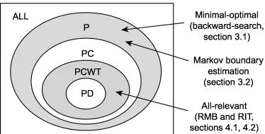
Figure 1: The distribution classes used. P, strictly positive; PC, strictly positive satisfying the com-position property; PCWT, strictly positive satisfying comcom-position and weak transitivity; PD, strictly positive and DAG-faithful. Arrows show classes where the various algorithms (right) are proved to be consistent.
model
X=x0+ε, ε∼N(0,σ).
Since the noise componentεis strictly positive over the domain of X , we immediately obtain f(x)>
0. A similar argument holds for binary data with Bernoulli noise, and indeed for any additive noise model with f(ε)>0. In general, the strictly positive restriction is considered reasonable whenever there is uncertainty about the data (Pearl, 1988). Note that the f(x)>0 criterion by definition only concerns the actual domain
X
. If the data distribution is known to be constrained for physical reasons to some compact set such as 0<X <1, then naturally f(x)>0 need not hold outside that set. Typical problems violating f(x)>0 involve noise-free data, such as inference of logic propositions (Valiant, 1984).In Section 4, we will consider the more narrow classes of strictly positive distributions (P) that also satisfy the composition property (PC), and those in PC that additionally satisfies the weak transitivity property (PCWT). See Appendix B for details on these properties. Although these re-strictions are more severe than f(x)>0, these classes still allow for many realistic models. For ex-ample, the jointly Gaussian distributions are known to be PCWT (Studen ´y, 2004). Also, the strictly positive and DAG-faithful distributions (PD) are contained in PCWT (Theorem 24, Appendix B). However, we hold that the PCWT class is more realistic than PD, since PCWT distributions will remain PCWT when a subset of the features are marginalized out (that is, are not observed), while PD distributions may not (Chickering and Meek, 2002).1 This is an important argument in favor of PCWT, as in many practical cases we cannot possibly measure all variables. An important example of this is gene expression data, which is commonly modelled by PD distributions (Friedman, 2004). However, it is frequently the case that not all genes can be measured, so that PCWT is a more realis-tic model class. Of course, these arguments also apply to the larger PC class. Figure 1 summarizes the relations between the distribution classes discussed in this section.
2.2 Classifiers, Risk and Optimality
A classifier is defined as a function g(x):
X
7→Y
, predicting a category y for each observed example x. The ”goodness” of a classifier is measured as follows.Definition 2 (risk) The risk R(g)of a classifier g is
R(g) =P(g(X)6=Y) =
∑
y∈Y
p(y)
Z
X1{g(x)6=y}f(x|y)dx, (1)
where 1{·}is the set indicator function.
For a given distribution f(x,y), an (optimal) Bayes classifier is one that minimizes R(g). It is easy to show that the classifier g∗that maximizes the posterior probability,
g∗(x) =
+1, P(Y =1|x)≥1/2
−1, otherwise , (2)
is optimal (Devroye et al., 1996). For strictly positive distributions, g∗(x) is also unique, except on zero-measure subsets of
X
(above, the arbitrary choice of g∗(x) = +1 at the decision boundary p(y|x) =1/2 is such a zero-measure set). This uniqueness is important for our results, so for completeness we provide a proof in Appendix A (Lemma 19). From now on, we speak of the optimal classifier g∗for a given f .2.3 Feature Relevance Measures
Much of the theory of feature selection is centered around various definitions of feature relevance. Unfortunately, many authors use the term ”relevant” casually and without a clear definition, which has caused much confusion on this topic. Defining relevance is not trivial, and there are many proposed definitions capturing different aspects of the concept; see for example Bell and Wang (2000) for a recent survey. The definitions considered in this paper are rooted in the well-known concept of (probabilistic) conditional independence (Pearl, 1988, sec. 2.1).
Definition 3 (conditional independence) A variable Xi is conditionally independent of a variable
Y given (conditioned on) the set of variables S⊂X iff it holds that
P p(Y|Xi,S) =p(Y|S)
=1.
This is denoted Y ⊥Xi|S.
In the above, the P(. . .) =1 is a technical requirement allowing us to ignore pathological cases where the posterior differs on zero-measure sets. Conditional independence is a measure of ir-relevance, but it is difficult to use as an operational definition since this measure depends on the conditioning set S. For example, a given feature Xi can be conditionally independent of Y given
S= /0 (referred to as marginal independence), but still be dependent for some S6= /0. The well-known XOR problem is an example of this. Two well-well-known relevance definitions coping with this problem were proposed by John et al. (1994).
Definition 4 (strong and weak relevance) A feature Xi is strongly relevant to Y iff Y6⊥Xi|Ri. A
feature Xi is weakly relevant to Y iff it is not strongly relevant, but satisfies Y6⊥Xi|S for some set
Informally, a strongly relevant feature carries information about Y that cannot be obtained from any other feature. A weakly relevant feature also carries information about Y , but this information is ”redundant”—it can also be obtained from other features. Using these definitions, relevance and irrelevance of a feature to a target variable Y are defined as
Definition 5 (relevance) A feature Xiis relevant to Y iff it is strongly relevant or weakly relevant to
Y.A feature Xiis irrelevant to Y iff it is not relevant to Y.
Finally, we will need the following definition of relevance with respect to a classifier.
Definition 6 A feature Xiis relevant to a classifier g iff
P(g(Xi,Ri)6=g(Xi0,Ri))>0,
where Xi,Xi0are independent and identically distributed.
This definition states that in order to be considered ”relevant” to g, a feature X must influence the value of g(x) with non-zero probability. It is a probabilistic version of that given by Blum and Langley (1997). Note that here, Xiand Xi0are independent samplings of the feature Xi; hence their
distributions are identical and determined by the data distribution f(x,y). In the next section, we examine the relation between this concept and the relevance measures in Definition 4.
3. The Minimal-Optimal Problem
In practise, the data distribution is of course unknown, and a classifier must be induced from the training data Dl ={(x(i),y(i))}l
i=1 by an inducer, defined as a function I :(
X
×Y
)l 7→G
, whereG
is some space of functions. We say that an inducer is consistent if the induced classifier I(Dl)converges in probability to g∗as the sample size l tends to infinity,
I(Dl)−→P g∗.
Consistency is a reasonable necessary criterion for a sound inducer, and has been verified for a wide variety of algorithms (Devroye et al., 1996). Provided that the inducer used is consistent, we can address the feature selection problem asymptotically by studying the Bayes classifier. We therefore define the optimal feature set as follows.
Definition 7 TheMINIMAL-OPTIMALfeature set S∗is defined as the set of features relevant to the Bayes classifier g∗(in the sense of Definition 6).
Clearly, S∗ depends only on the data distribution, and is the minimal feature set that allows for optimal classification; hence its name. Since g∗is unique for strictly positive distributions (Lemma 19), it follows directly from Definition 6 that S∗is then also unique. Our first theorem provides an important link between theMINIMAL-OPTIMALset and the concept of strong relevance.
X1
- 2 - 1 0 1 2
- 2 - 1
0
1
2
X2 ( w e a k l y r e l e v a n t )
( s t r o n g l y r e l e v a n t )
R i s k
# s a m p l e s a l l f e a t u r e s
s t r o n g l y r e l e v a n t f e a t u r e s
2 0 4 0 6 0 8 0 1 0 0 0 . 0 2
0 . 0 6 0 . 1 0
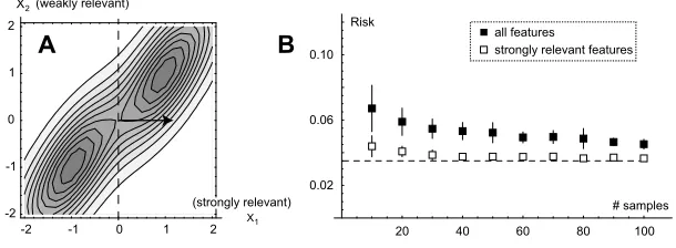
Figure 2: A: The example density f(x2i−1,x2i)given by (4). Here, X1 is strongly relevant and X2 weakly relevant. Arrow and dashed line indicates the optimal separating hyperplane. B: The risk functional R(g) for a linear SVM trained on all relevant features (filled boxes) vs. on strongly relevant features only (open boxes), for the 10-dimensional distribution (4). Average and standard deviation over 20 runs are plotted against increasing sample size. The Bayes risk (dashed line) is R(g∗) =0.035.
Proof Since f is strictly positive, g∗ is unique by Lemma 19 (Appendix A). Consider any feature Xi relevant to g∗, so that P(g∗(Xi,Ri)6=g∗(Xi0,Ri))>0 by Definition 6. From the form (2) of the
Bayes classifier, we find that
g∗(xi,ri)6=g∗(x0i,ri)⇒p(y|xi,ri)6=p(y|x0i,ri) (3)
everywhere except possibly on the decision surface{x : p(y|x) =1/2}. But this set has zero proba-bility due to assumption (ii) of Definition 1. Therefore,
P(p(Y|Xi,Ri)=6 p(Y|Xi0,Ri))≥P(g∗(Xi,Ri)6=g∗(Xi0,Ri))>0.
By Lemma 20 this is equivalent to P(p(Y|Xi,Ri) = p(Y|Ri))<1, which is the same as Y 6⊥Xi|Ri.
Hence, Xiis strongly relevant.
Note that uniqueness of g∗is required here: if there would exist a different Bayes classifier g0, the implication (3) would not hold. Theorem 8 is important because it asserts that we may safely ignore weakly relevant features, conditioned on the assumption f(x)>0. This leads to more efficient (polynomial-time) algorithms for finding S∗ for such problems. We will explore this consequence in Section 3.3.
An example illustrating Theorem 8 is given in Figure 2. Here, f is a 10-dimensional Gaussian mixture
f(x1, . . . ,x10,y)∝ 5
∏
i=1
e−98((x2i−1−y)
2+(x
2i−1−x2i)2). (4)
it is easy to verify directly from (4) that X2,X4, . . . ,X10are weakly relevant: considering for example the pair(X1,X2), we have
p(y|x1,x2) =
f(x1,x2,y) f(x1,x2)
=
1+exp
−9
8((x1+y) 2−(x
1−y)2) −1
=
1+exp
−9x1y
2 −1
which depends only on x1, so X2is weakly relevant. The Bayes classifier is easy to derive from the condition p(y|x)>1/2 (Equation 2) and turns out to be g∗(x) =sgn(x1+x3+x5+x7+x9), so that S∗={1,3,5,7,9}as expected.
For any consistent inducer I, Theorem 8 can be treated as an approximation for finite (but suffi-ciently large) samples. If this approximation is fair, we expect that adding weakly relevant features will degrade the performance of I, since the Bayes risk must be constant while the design cost must increase (Jain and Waller, 1978). To illustrate this, we chose I to be a linear, soft-margin support vector machine (SVM) (Cortes and Vapnik, 1995) and induced SVM classifiers from training data sampled from the density (4), with sample sizes l=10,20, . . . ,100. Figure 2B shows the risk of g=I(Dl)and gS∗ =IS∗(DlS∗)(here and in what follows we take gS∗, IS∗, and DlS∗ to mean
classi-fiers/inducers/data using only the features in S∗). The SVM regularization parameter C was chosen by optimization over a range 10−2, . . . ,102; in each case, the optimal value was found to be 102. We found that IS∗ does outperform I, as expected. The risk functional R(g)was calculated by numerical
integration of Equation (1) for each SVM hyperplane g and averaged over 20 training data sets. Clearly, adding the weakly relevant features increases risk in this example.
As the following example illustrates, the converse of Theorem 8 is false: there exist strictly positive distributions where even strongly relevant features are not relevant to the Bayes classifier.
Example 1 Let
X
= [0,1],Y
={−1,+1}, f(x)>0 and p(y=1|x) =x/2. Here X is clearly strongly relevant. Yet, X is not relevant to the Bayes classifier, since we have p(y=1|x)<1/2 almost everywhere (except at x=1). We find that g∗(x) =−1 and R(g∗) =P(Y=1).Clearly, this situation occurs whenever a strongly relevant feature Xiaffects the value of the posterior
p(y|x)but not the Bayes classifier g∗(because the change in p(y|x)is not large enough to alter the decision of g∗(x)). In this sense, relevance to the Bayes classifier is stronger than strong relevance.
3.1 Related Work
The relevance concepts treated above have been studied by several authors. In particular, the relation between the optimal feature set and strong vs. weak relevance was treated in the pioneering study by Kohavi and John (1997), who concluded from motivating examples that ”(i) all strongly relevant features and (ii) some of the weakly relevant ones are needed by the Bayes classifier”. As we have seen in Example 1, part (i) of this statement is not correct in general. Part (ii) is true in general, but Theorem 8 shows that this is not the case for the class of strictly positive f , and therefore it is rarely true in practise.
which the latter is deemed to be important for the Bayes classifier. However, Yu & Liu consider arbitrary distributions; for strictly positive distributions however, it is easy to see that all weakly relevant features are also ”redundant” in their terminology, so that their distinction is not useful in this case.
3.2 Connections with Soft Classification
A result similar to Theorem 8 have recently been obtained for the case of soft (probabilistic) clas-sification (Hardin et al., 2004; Tsamardinos and Aliferis, 2003). In soft clasclas-sification, the objective is to learn the posterior p(y|x)instead of g∗(x). By Definition 6, the features relevant to the optimal soft classifier p(y|x)satisfies
P(p(Y|Xi,Ri)=6 p(Y|Xi0,Ri))>0
which is equivalent to P(p(Y|Xi,Ri)6=p(Y|Ri))>0 by Lemma 20. Thus, the features relevant to
p(y|x)are exactly the strongly relevant ones, so the situation in Example 1 does not occur here. When learning soft classifiers from data, a feature set commonly encountered is the Markov boundary of the class variable, defined as the minimal feature set required to predict the posterior. Intuitively, this is the soft classification analogue of MINIMAL-OPTIMAL. The following theorem given by Pearl (1988, pp. 97) shows that this set is well-defined for strictly positive distributions.2 Theorem 9 (Markov boundary) For any strictly positive distribution f(x,y), there exists a unique minimal set M⊆X satisfying Y ⊥X\M|M. This minimal set is called the Markov boundary of the variable Y (with respect to X ) and denoted M(Y|X).
Tsamardinos & Aliferis recently proved that for the PD distribution class (see Figure 1), the Markov boundary coincides with the set of strongly relevant features (Tsamardinos and Aliferis, 2003). However, as explained in Section 2.1, the PD class is too narrow for many practical applications. Below, we generalize their result to any positive distribution to make it more generally applicable.
Theorem 10 For any strictly positive distribution f(x,y), a feature Xi is strongly relevant if and
only if it is in the Markov boundary M=M(Y|X)of Y .
Proof First, assume that Xiis strongly relevant. Then Y6⊥Xi|Ri, which implies M6⊆Ri, so Xi∈M.
Conversely, fix any Xi∈M and let M0=M\ {Xi}. If Xiis not strongly relevant, then Y⊥Xi|Ri, and
by the definition of the Markov boundary, Y⊥X\M|M. We may rewrite this as
Y⊥Xi|M0∪X\M
Y⊥X\M|M0∪ {Xi}.
The intersection property (Theorem 25, Appendix B) now implies Y⊥X\M0|M0. Hence, M0 is a Markov blanket smaller than M, a contradiction. We conclude that Xiis strongly relevant.
The feature set relations established at this point for strictly positive distributions are summarized in Figure 3.
Irrelevant features weakly relevant features strongly relevant
features = markov blanket
= features relevant to the posterior p(y|x)
minimal-optimal set
all-relevant set = strongly + weakly relevant features
Figure 3: The identified relations between feature sets for strictly positive distributions. The circle represents all features. The dotted line (MINIMAL-OPTIMAL) denotes a subset, while the solid lines denote a partition into disjoint sets.
3.3 Consistent Polynomial Algorithms
By limiting the class of distributions, we have simplified the problem to the extent that weakly relevant features can be safely ignored. In this section, we show that this simplification leads to polynomial-time feature selection (FS) algorithms. A FS algorithm can be viewed as a function
Φ(Dl):(
X
×Y
)l 7→2X, where 2X denotes the power-set of X . For finite samples, the optimalΦdepends on the unknown data distribution f and the inducer I (Tsamardinos and Aliferis, 2003). Asymptotically however, we may use consistency as a reasonable necessary criterion for a ”cor-rect” algorithm. In analogue with consistency of inducers, we define a FS algorithmΦ(Dl) to be consistent if it converges in probability to theMINIMAL-OPTIMALset,
Φ(Dl)−→P S∗.
Conveniently, consistency of Φ depends only on the data distribution f . Next, we propose a polynomial-time FS algorithm and show that it is consistent for any strictly positive f . As before, feature sets used as subscripts denote quantities using only those features.
Theorem 11 Take any strictly positive distribution f(x,y)and let ˆc(DlS)be a real-valued criterion function such that, for every feature subset S,
ˆ
c(DlS)−→P c(S), (5)
where c(S)depends only on the distribution f(x,y)and satisfies
c(S)<c(S0) ⇐⇒ R(g∗S)<R(g∗S0). (6)
Then the feature selection method
Φ(Dl) ={i : ˆc(DRli)>cˆ(Dl) +ε}
Proof Since f is strictly positive, S∗is unique by Lemma 19. By Definition 7 and the assumption (6) it holds that Xi∈S∗ iff c(X)<c(Ri). First consider the case Xi∈S∗. Fix anε∈(0,η)and let ε0=min{(η−ε)/2,ε/2}. Choose anyδ>0. By (5) there exist an l
0such that for all l>l0, P
max
S |cˆ(D l
S)−c(S)|>ε0
≤δ/2n
Note that since the power-set 2X is finite, taking the maxima above is always possible even though (5) requires only point-wise convergence for each S. Therefore the events (i) ˆc(DlX)<c(X) +ε0and
(ii) ˆc(DlRi)>c(Ri)−ε0 both have probability at least 1−δ/2n. Subtracting the inequality (i) from
(ii) yields
ˆ
c(DlRi)−cˆ(DlX) > c(Ri)−c(X)−2ε0
≥ c(Ri)−c(X)−(η−ε)≥ε.
Thus, for every l>l0,
P(Xi∈Φ(Dl)) = P(cˆ(DlRi)−cˆ(D
l X)>ε)
≥ P
ˆ
c(DlX)<c(X) +ε0 ∧ cˆ(DlRi)>c(Ri)−ε0
≥ P
ˆ
c(DlX)<c(X) +ε0+P
ˆ
c(DlRi)>c(Ri)−ε0
−1
≥ 1−δ/n.
For the converse case Xi6∈S∗, note that since c(X) =c(Ri),
P(Xi∈Φ(Dl)) = P
ˆ
c(DlRi)−cˆ(DlX)>ε
≤ P(|cˆ(DRli)−c(Ri)|+|c(X)−cˆ(DlX)|>ε)
≤ P|cˆ(DlRi)−c(Ri)|> ε
2 ∨ |c(X)−cˆ(D
l X)|>
ε
2
≤ P|cˆ(DlRi)−c(Ri)|>ε0
+P|c(X)−cˆ(DlX)|>ε0≤δ/n
where in the last line we have usedε0≤ε/2. Putting the pieces together, we obtain
P(Φ(Dl) =S∗) = P(Φ(Dl)⊇S∗ ∧ Φ(Dl)⊆S∗)
= P(∀i∈S∗: Xi∈Φ(Dl) ∧ ∀i6∈S∗: Xi6∈Φ(Dl))
≥ |S∗|(1−δ/n) + (n− |S∗|)(1−δ/n)−(n−1) =1−δ.
Sinceδwas arbitrary, the required convergence follows.
The algorithm Φ evaluates the criterion ˆc precisely n times, so it is clearly polynomial in n provided that ˆc is. The theorem applies to both filter and wrapper methods, which differ only in the choice of ˆc(DlS)(Kohavi and John, 1997). To apply the theorem in a particular case, we need only verify that the requirements (5) and (6) hold. For example, let I be the k-NN rule with training data
Dl/2={(X1,Y1), . . . ,(Xl/2,Yl/2)} and let ˆR be the usual empirical risk estimate on the remaining
samples{(Xl/2+1,Yl/2+1), . . . ,(Xl,Yl)}. Provided k is properly chosen, this inducer is known to be
universally consistent,
P(R(IS(D l/2
S ))−R(g∗S)>ε)≤2e−lε
2/(144γ2
S)
whereγSdepends on|S|but not on l (Devroye et al., 1996, pp. 170). Next, with a test set of size l/2, the empirical risk estimate satisfies
∀g : P(|Rˆ(g)−R(g)|>ε)≤2e−lε2
(Devroye et al., 1996, pp. 123). We choose ˆc(Dl
S) =Rˆ(IS(DSl/2))and c(S) =R(g∗S), so that (6) is
immediate. Further, this ˆc(DlS)satisfies
P
|cˆ(DlS)−c(S)|>ε=P
|Rˆ(IS(Dl/2
S ))−R(g ∗ S)|>ε
≤P|Rˆ(IS(Dl/2
S ))−R(IS(DSl/2))|+|R(IS(DlS/2))−R(g∗S)|>ε
≤P|Rˆ(IS(Dl/2
S ))−R(IS(DlS/2))|> ε
2
+P|R(IS(DSl/2))−R(g∗S)|>
ε
2
≤2e−lε2/4+2e−lε2/(576γ2S)→0
for every S as required by (5), and is polynomial in n. Therefore this choice defines a polynomial-time, consistent wrapper algorithm Φ. Note that we need only verify the point-wise convergence (5) for any given ˆc(S), which makes the application of the theorem somewhat easier. Similarly, other consistent inducers and consistent risk estimators could be used, for example support vector machines (Steinwart, 2002) and the cross-validation error estimate (Devroye et al., 1996, chap. 24). The FS method Φ described in Theorem 11 is essentially a backward-elimination algorithm. With slight modifications, the above shows that many popular FS methods that implement variants of backward-search, for example Recursive Feature Elimination (Guyon et al., 2002), are in fact consistent. This provides important evidence of the soundness of these algorithms.
In contrast, forward-search algorithms are not consistent even for strictly positive f . Starting a with feature set S, forward-search would find the feature set S0=S∪ {Xi}(that is, add feature Xi) iff
ˆ
c(DlS0)<cˆ(DlS). But it may happen that R(g∗S0)≮R(g∗S)even though S0is contained in S∗. Therefore,
forward-search may miss features in S∗. The ”noisy XOR problem” (Guyon and Elisseeff, 2003, pp. 1116) is an example of a strictly positive distribution with this property.
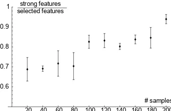
A simple example illustrating Theorem 11 is shown in Figure 4. We implemented the feature se-lection methodΦdefined in the theorem, and again used the data density f from Equation (4). Also here, we employed a linear SVM as inducer. We used the leave-one-out error estimate (Devroye et al., 1996) as ˆR. As sample size increases, we find that the fraction of strongly relevant features selected approaches 1, confirming thatΦ(Dl)−→P S∗. Again, this emphasizes that asymptotic results can serve as good approximations for reasonably large sample sizes.
20 4 0 6 0 8 0 1 0 0 1 20 1 4 0 1 6 0 1 8 0 20 0 0 . 6
0 . 7 0 . 8 0 . 9
1 s t r o n g f e a t u r e s s e l e c t e d f e a t u r e s
# s a m p l e s
Figure 4: A feature selection example on a 10-dimensional density with 5 strongly and 5 weakly relevant features (Equation 4). Averaged results of 50 runs are plotted for samples sizes
20, . . . ,200. Error bars denote standard deviations.
Data set l×n No FS Φε=0 RELIEF FCBF Breast cancer 569×30 8 9(7) 69(8) 62(2) Ionosphere 351×34 11 9(14) 16(26) 14(5) Liver disorder 345×6 36 39(5) −(0) 43(2) E.Coli 336×7 36 20(5) 43(1) 57(1) P.I. Diabetes 768×8 33 36(7) 35(1) 35(1) Spambase 4601×57 12 17(39) 25(26) 40(4)
we conducted some experiments usingΦ on a set of well-known data sets from the UCI machine learning repository (Newman et al., 1998) to demonstrate empirically that weakly relevant features do not contribute to classifier accuracy. We used a 5-NN classifier together with a 10-fold cross-validation error estimate for the criterion function ˆc. For each case we estimated the final accuracy by holding out a test set of 100 examples. Statistical significance was evaluated using McNemar’s test (Dietterich, 1998). We setε=0 in this test, as we were not particularly concerned about false positives. For comparison we also tried the RELIEFalgorithm (Kira. and Rendell, 1992) and the FBCF algorithm by Yu and Liu (2004), both of which are based on the conjecture that weakly relevant features may be needed. We found thatΦnever increased test error significantly compared to the full data set, and significantly improved the accuracy in one case (Table 1). The FCBF and Relief algorithms significantly increased the test error in five cases. Overall, these methods selected very few features (in one case, RELIEF selected no features at all) using the default thresholds recommended by the original papers (for FCBF,γ=n/log n and for RELIEF,θ=0, in the notation of each respective paper; these correspond to theεparameter of theΦalgorithm).
In the case of the P.I. Diabetes set, Φ seems to select redundant features, which at first might seem to contradict our theory. This may happen for two reasons. First, atε=0, theΦ algorithm is inclined to to include false positives (redundant features) rather than risk any false negatives. Second, it is possible that some of these features are truly in S∗, even though the reduction in classification error is too small to be visible on a small test set.
Theorem 10 also has implications for algorithmic complexity in the case of soft classification. To find the Markov boundary, one need now only test each Xi for strong relevance, that is, for the
conditional independence Y ⊥Xi|XRi. This procedure is clearly consistent and can be implemented in polynomial time. It is not very practical though, since these tests have very limited statistical power for large n due to the large conditioning sets Ri. However, realistic solutions have recently
been devised for more narrow distribution classes such as PC, yielding polynomial and consistent algorithms (Pe˜na et al., 2005; Tsamardinos and Aliferis, 2003).
4. The All-Relevant Problem
Recently, feature selection has received much attention in the field of bioinformatics, in particular in gene expression data analysis. Although classification accuracy is an important objective also in this field, many researchers are more interested in the ”biological significance” of features (genes) that depend on the target variable Y (Slonim, 2002). As a rule, biological significance means that a gene is causally involved in the biological process of interest. It is imperative to understand that this biological significance is very different from that in Definition 5. Clearly, genes may be useful for predicting Y without being causally related, and may therefore be irrelevant to the biologist.
Therefore, it is desirable to identify all genes relevant to the target variable, rather than the set S∗, which may be more determined by technical factors than by biological significance. Hence, we suggest that the following feature set should be found and examined.
Definition 12 For a given data distribution, theALL-RELEVANTfeature set SAis the set of features relevant to Y in the sense of Definition 5.
To the best of our knowledge, this problem has not been studied. We will demonstrate that because SA includes weakly relevant features (Figure 3), theALL-RELEVANTproblem is much harder than
MINIMAL-OPTIMAL. In fact, the problem of determining whether a single feature Xi is weakly
relevant requires exhaustive search over all 2n subsets of X , even if we restrict ourselves to strictly positive distributions.
Theorem 13 For a given feature Xi and for every S⊆Ri, there exists a strictly positive f(x,y)
satisfying
Y6⊥Xi|S ∧ ∀S06=S : Y ⊥Xi|S0. (7)
Proof Without loss of generalization we may take i=n and S=X1, . . .Xk, k=|S|. Let S∪ {Xk+1} be distributed as a k+1-dimensional Gaussian mixture
f(s,xk+1|y) = 1
|My|µ∈M
∑
y
N(s,xk+1|µ,Σ),
My = {µ∈ {1,0}k+1: µ1⊕ · · · ⊕µk+1= (y+1)/2},
where⊕is the XOR operator (Myis well-defined since⊕is associative and commutative). This
dis-tribution is a multivariate generalization of the ”noisy XOR problem” (Guyon and Elisseeff, 2003). It is obtained by placing Gaussian densities centered at the corners of a k+1-dimensional hyper-cube given by the sets My, for y=±1. It is easy to see that this gives Y6⊥Xk+1|S and Y⊥Xk+1|S0 if S0⊂S. Next, let Xi+1=Xi+εfor k<i<n, whereεis some strictly positive noise distribution.
Then it holds that Y6⊥Xi|S for k<i<n, and in particular Y6⊥Xn|S. But it is also clear that Y⊥Xn|S0 for S0⊃S, since every such S0 contain a better predictor Xi,k<i<n of Y . Taken together, this is
equivalent to (7), and f is strictly positive.
This theorem asserts that the conditioning set that satisfies the relation Y6⊥Xi|S may be
com-pletely arbitrary. Therefore, no search method other than exhaustively examining all sets S can possibly determine whether Xi is weakly relevant. Since ALL-RELEVANT requires that we
deter-mine this for every Xi, the following corollary is immediate.
Corollary 14 The all-relevant problem requires exhaustive subset search.
Exhaustive subset search is widely regarded as an intractable problem, and no polynomial algo-rithm is known to exist. This fact is illustrative in comparison with Theorem 8;MINIMAL-OPTIMAL is tractable for strictly positive distributions precisely because S∗does not include weakly relevant features.
Algorithm 1: Recursive independence test (RIT) Input: target node Y , features X
Let S=/0;
foreach Xi∈X do
if Xi6⊥Y|/0then
S=S∪ {Xi};
end end
foreach Xi∈S do
S=S∪RIT(Xi,X\S);
end return S
4.1 Recursive Independence Test
A simple, intuitive method for solving ALL-RELEVANT is to test features pairwise for marginal dependencies: first test each feature against Y , then test each feature against every variable found to be dependent on Y , and so on, until no more dependencies are found (Algorithm 1). We refer to this algorithm as Recursive Independence Testing (RIT). We now prove that the RIT algorithm is consistent (converges to SA) for PCWT distributions, provided that the test used is consistent.
Theorem 15 For any PCWT distribution, let R denote the set of variables Xk∈X for which there
exists a sequence Z1m ={Z1, . . . ,Zm} between Z1 =Y and Zm =Xk such that Zi6⊥Zi+1|/0, i=
1, . . . ,m−1. Then R=SA.
Proof Let I =X\R and fix any Xk ∈I. Since Y⊥Xk|/0 and Xi⊥Xk|/0 for any Xi∈R, we have {Y} ∪R⊥I|/0by the composition property. Then Y⊥Xk|S for any S⊂X\ {Xk,Y}by the weak union
and decomposition properties, so Xkis irrelevant; hence, SA⊆R.
For the converse, fix any Xk ∈R and let Zm1 ={Z1, . . . ,Zm} be a shortest sequence between Z1=Y and Zm=Xk such that Zi6⊥Zi+1|/0 for i=1, . . . ,m−1. Then we must have Zi⊥Zj|/0 for
j>i+1, or else a shorter sequence would exist. We will prove that Z16⊥Zm|Z2m−1 for any such shortest sequence, by induction over the sequence length. The case m=2 is trivial. Consider the case m=p. Assume as the induction hypothesis that, for any i,j<p and any chain Zii+j of length
j, it holds that Zi6⊥Zi+j|Zii++1j−1. By the construction of the sequence Z1mit also holds that
Z1⊥Zi|/0, 3≤i≤m =⇒ Z1⊥Z3i|/0 (8)
(composition)
=⇒ Z1⊥Zi|Zi−3 1. (9)
(weak union)
Now assume to the contrary that Z1⊥Zp|Z2p−1. Together with (9), weak transitivity implies Z1⊥Z2|Z3p−1 ∨ Z2⊥Zp|Z3p−1.
Algorithm 2: Recursive Markov Boundary (RMB) Input: target node Y , data X , visited nodes V Let S=M(Y|X), the Markov blanket of Y in X ; foreach Xi∈S\V do
S=S∪RMB(Y,X\ {Xi},V); V =V∪S
end return S
hence Z16⊥Zp|Z2p−1, which completes the induction step. Thus Xk is relevant and R⊆SA. The
theorem follows.
Corollary 16 For any PCWT distribution and any consistent marginal independence test, the RIT algorithm is consistent.
Proof Since the test is consistent, the RIT algorithm will discover every sequence Z1m={Z1, . . . ,Zm}
between Z1=Y and Zm=Xk with probability 1 as l→∞. Consistency follows from Theorem 15.
Since the RIT algorithm makes up to n=|X|tests for each element of R found, in total RIT will evaluate no more than n|R|tests. Thus, for small R the number of tests is approximately linear in n, although the worst-case complexity is quadratic.
There are many possible alternatives as to what independence test to use. A popular choice in Bayesian networks literature is Fisher’s Z-test, which tests for linear correlations and is consis-tent within the family of jointly Gaussian distributions (Kalisch and B ¨uhlmann, 2005). Typically, for discrete Y a different test is needed for testing Y⊥Xi|/0 than for testing Xi⊥Xj. A
reason-able choice is Student’s t-test, which is consistent for jointly Gaussian distributions (Casella and Berger, 2002). More general independence tests can be obtained by considering correlations in kernel Hilbert spaces, as described by Gretton et al. (2005).
4.2 Recursive Markov Boundary
In this section we propose a second algorithm forALL-RELEVANTcalled Recursive Markov Bound-ary (RMB), based on a given consistent estimator of Markov boundaries of Y . Briefly, the RMB algorithm first estimates M(Y|X), then estimates M(Y|X\ {Xi}) for each Xi ∈M(Y|X), and so on
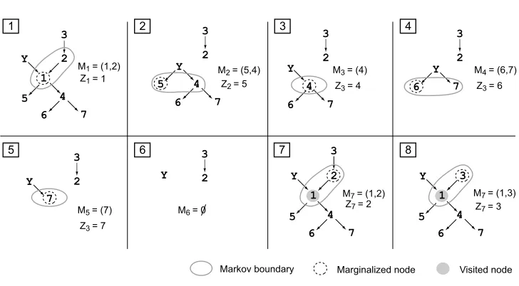
recursively until no more nodes are found (Algorithm 2). For efficiency, we also keep track of pre-viously visited nodes V to avoid visiting the same nodes several times. We start the algorithm with RMB(Y,X,V = /0). A contrived example of the RMB algorithm for a PD distribution is given in Figure 5.
Definition 17 An independence map (I-map) over a set of features X ={X1, . . . ,Xn} is an
undi-rected graph G over X satisfying
R⊥GS|T =⇒ R⊥S|T
where R,S,T are disjoint subsets of X and⊥Gdenotes vertex separation in the graph G, that is,
R⊥GS|T holds iff every path in G between R and S contains at least one Xi∈T . An I-map is minimal
if no subgraph G0of G (over the same nodes X ) is an I-map.
Note that we only consider the minimal I-map over the features X (not over X∪ {Y}), since in this case, the minimal I-map is unique for any strictly positive distribution (Pearl, 1988).
Theorem 18 For any PCWT distribution such that a given estimator M(Y|S)of the Markov bound-ary of Y with respect to a feature set S is consistent for every S⊆X , the RMB algorithm is consistent.
Proof For every S⊆X , the marginal distribution over S,Y is strictly positive, and therefore every Markov boundary M(Y|S)is unique by corollary 26 (Appendix B). Let G be the minimal I-map over the features X , and let M1=M(X|Y). Fix an Xk in SA. If Xk∈M1, we know that Xk is found
by RMB. Otherwise, by Lemma 22, there exists a shortest path Z1min G between some Z1∈M1and Zm=Xk. We prove by induction over m that RMB visits every such path. The case m=1 is trivial.
Let the induction hypothesis be that Zpis visited. For Zp+1, Lemma 22 implies Y6⊥Zp+1|X\Z1p+1. Since Zpis visited, RMB will also visit all nodes in Mp+1=M(Y|X\Z1p). However, Mp+1contains Zp+1, because it contains all Xisatisfying Y6⊥Xi|X\Z1p\ {Xi}by Theorem 10.
It is easy to see from algorithm 2 that the RMB algorithm requires computing |SA| Markov
blankets. We might attempt to speed it up by marginalizing out several nodes at once, but in that case we cannot guarantee consistency. A general algorithm for estimating Markov boundaries is given by Pe˜na et al. (2005). This estimator is consistent in the PC class, so it follows that RMB is consistent in PCWT in this case (see Figure 1).
At first sight, RMB may seem more computationally intensive that RIT. However, since the Markov boundary is closely related to S∗(see Section 3.2), we anticipate that RMB may be imple-mented using existing FS methods. In particular, for distribution classes where the Markov bound-ary coincides with theMINIMAL-OPTIMALset S∗, one may compute M(Y|X)using any FS method that consistently estimates S∗. For example, this property holds for the well-known class of jointly Gaussian distributions f(x|y) =N(x|yµ,Σ)with p(y) =1/2. To see this, note that the posterior and Bayes classifier are given by
p(y|x) =
1+exp{−2yµTΣ−1x}−1
,
g∗(x) = sgn(µTΣ−1x).
Clearly, both g∗(x) and p(y|x) are constant with respect to an xi iff(µTΣ−1)i=0. Thus, in this
case S∗ equals the Markov boundary. SVM-based FS methods are one attractive option, as there exist efficient optimization methods for re-computation of the SVM solution after marginalization (Keerthi, 2002).
4.3 Related Work
Y 3 2 4 5 6 7 Y 4 5 6 7
Ma r k o v b o u n d a r y Ma r g i n a l i z e d n o d e V i s i t e d n o d e
M1 = ( 1 , 2 )
M7 = ( 1 , 2 )
M2 = ( 5 , 4 )
Z 1 = 1 Z
2 = 5
Y
4
6 7
M3 = ( 4 )
Z 3 = 4
Y
6 7
M4 = ( 6 , 7 )
Z 3 = 6
Y
7
M5 = ( 7 )
Z 3 = 7
Z 7 = 2
Y
M6 = 0
1
5 6 7 8
2 3 3 4
2 3 2 3 2 3 2 3 2 Y 3 2 1 4 5 6 7 4 5 6 7 1 Y 3
M7 = ( 1 , 3 )
Z 7 = 3
1
Figure 5: A contrieved example of the RMB algorithm for a PD distribution faithful to the DAG shown in black arrows. Numbers denote the relevant features, Y denotes the target vari-able. As in Theorem 18, Mi denotes Markov boundaries and Zi denotes marginalized
nodes. Note that the marginal distributions from step 2 onwards may not be PD, so ab-sence of arrows should not be interpreted as independencies.
ALL-RELEVANTcan be solved by inferring a Bayesian network and then taking SA to be the
con-nected component of Y in that network. However, this is less efficient than our approach, since Bayesian network inference is asymptotically NP-hard, even in the very restricted PD class (Chick-ering et al., 2004). Certainly, such a strategy seems inefficient as it attempts to ”solve a harder problem as an intermediate step” (by inferring a detailed model of the data distribution merely to find the set SA), thus violating Vapnik’s famous principle (Vapnik, 2000, pp. 39).
On the other hand, several methods have been proposed for solving MINIMAL-OPTIMAL that in fact attempt to find all relevant features, since they do not assume f >0 and therefore cannot rule out the weakly relevant ones. These include FOCUS(Almuallim and Dietterich, 1991), which considers the special case of binary
X
and noise-free labels; RELIEF (Kira. and Rendell, 1992), a well-known approximate procedure based on nearest-neighbors; Markov blanket filtering (Koller and Sahami, 1996; Yu and Liu, 2004), which considers the special case of marginal dependencies (and is therefore fundamentally different from RMB, despite the similar name). All known methods are either approximate or have exponential time-complexity.5. Conclusion
restriction to strictly positive distributions is sufficient for the MINIMAL-OPTIMALproblem to be tractable (Figure 1). Therefore, we conclude that it is tractable in most practical settings.
We have also identified a different feature selection problem, that of discovering all relevant fea-tures (ALL-RELEVANT). This problem is much harder than MINIMAL-OPTIMAL, and has hitherto received little attention in the machine learning field. With the advent of major new applications in the bioinformatics field, where identifying features per se is often a more important goal than building accurate predictors, we anticipate that ALL-RELEVANTwill become a very important re-search problem in the future. We have herein provided a first analysis, proved that the problem is intractable even for strictly positive distributions, and proposed two consistent, polynomial-time algorithms for more restricted classes (Figure 1). We hope that these results will inspire further research in this novel and exciting direction.
Acknowledgments
We would like to thank the editor and the anonymous reviewers for helpful comments and insight, as well as for pointing out an initial problem with the proof of Lemma 19 and also suggesting a rem-edy to that problem. We also thank Timo Koski, Department of Mathematics, Link ¨oping University for proof-reading and Peter Jonsson, Department of Computer and Information Science, Link ¨oping University for valuable discussions. This work was supported by grants from the Swedish Foun-dation for Strategic Research (SSF), the Ph.D. Programme in Medical Bioinformatics, the Swedish Research Council (VR-621-2005-4202), Clinical Gene Networks AB and Link ¨oping University.
Appendix A. Lemmas
For completeness, we here give a proof of the uniqueness of the Bayes classifier for strictly positive distributions.
Lemma 19 For any strictly positive distribution f(x,y), the Bayes classifier g∗ is unique in the sense that, for every classifier g, it holds that R(g) =R(g∗)iff the Lebesgue measure of{x : g(x)6=
g∗(x)}is zero.
Proof By Theorem 2.2 of Devroye et al. (1996), the risk of any classifier g can be written as
R(g) =R(g∗) +
Z
X
max
y p(y|x)−
1 2
1{g(x)6=g∗(x)}f(x)dx.
By property (ii) of Definition 1, we have maxyp(y|x)6=1/2 almost everywhere. Thus, the integral
is zero iff the Lebesgue measure of{x : g(x)6=g∗(x)}is zero.
Lemma 20 For any conditional distribution p(y|x), it holds that
P(p(Y|Xi,Ri) =p(Y|Xi0,Ri)) =1 ⇐⇒ P(p(Y|Xi,Ri) =p(Y|Ri)) =1
Proof Assume that the left-hand side holds. Then we must have
P(p(Y|Xi,Ri) =p0) =1 for some p0constant with respect to Xi. But
p(y|ri) =
f(ri,y)
f(ri)
=
R
Xip(y|x)f(x)
R
Xi f(x)
= p0
R
Xi f(x)
R
Xi f(x)
=p0
with probability 1, which implies the right-hand side. The converse is trivial.
The following lemmas are needed for the correctness proof for the RMB algorithm.
Lemma 21 Let f(x) be any PCWT distribution, so that a unique undirected minimal I-map G of f exists. Then, for any shortest path Z1m={Z1, . . .Zm} between Z1 and Zm in G, it holds that
Z16⊥Zm|X\Zm1.
Proof The proof is by induction. For m=2, the lemma follows immediately from the definition of the minimal I-map (Pearl, 1988). Also, it holds that
Zi6⊥Zi+1|X\ {Zi,Zi+1} (10) Zi⊥Zj|X\ {Zi,Zj}, j>i+1. (11)
Take any distinct Zii+1,Zk and assume that Zi⊥Zi+1|X\ {Zi,Zi+1,Zk}. Then Zi⊥ {Zi+1,Zk}|X\ {Zi,Zi+1,Zk}by contraction with (11), and therefore Zi⊥Zi+1|X\ {Zi,Zi+1}by weak union. This contradicts (10), so we conclude that
Zi6⊥Zi+1|X\ {Zi,Zi+1,Zk}. (12)
Next, take any sequence Zii+2. Applying (12), we obtain Zi6⊥Zi+1|X\Zii+2 and Zi+16⊥Zi+2|X\ Zii+2. Using weak transitivity implies either Zi6⊥Zi+2|X\Zii+2or Zi6⊥Zi+2|X\ {Zi,Zi+2}. The latter alternative contradicts (11), so we conclude
Zi6⊥Zi+2|X\Zii+2. (13)
Finally, take any Zi,Zj,Zk such that neither Zi,Zj nor Zj,Zk are consecutive in the path Zm1. Using (11) with intersection (Theorem 25) and decomposition (Theorem 23), we find
Zi⊥Zj|X\ {Zi,Zj}
Zj⊥Zk|X\ {Zj,Zk}
=⇒ Zi⊥Zj|X\ {Zi,Zj,Zk}. (14)
Equations (12),(13) and (14) show that the properties (10) and (11) hold also for the shortened path
Z10, . . . ,Zm−0 1given by Z01=Z1 and Zi0=Zi+1,2≤i<m (removing Z2). The lemma follows from
(10) by induction.
Lemma 22 For any PCWT distribution f(x,y), a feature Xk is relevant iff there exists a path
Z1m={Z1, . . .Zm} in the minimal I-map of f(x) between some Z1∈M=M(Y|X) and Zm=Xk.
Proof If Zm∈M (that is, m=1), the lemma is trivial. Consider any Zm∈/ M. First, assume that
there exists no path Z1m. Then Zm⊥M|S for any S⊆X\M\ {Zm}by Lemma 21. Fix such an S.
Since Zm⊥Y|M∪S, contraction and weak union gives Zm⊥M|{Y} ∪S. Again using Zm⊥M|S,
weak transitivity gives
Zm⊥Y|S ∨ Y⊥M|S.
The latter alternative is clearly false; we conclude Zm⊥Y|S. Next, fix any S0⊆M. By
decomposi-tion, Zm⊥M|S =⇒ Zm⊥S0|S. Combining with the above result, by the composition property
Zm⊥S0|S
Zm⊥Y|S
=⇒ Zm⊥ {Y} ∪S0|S.
Finally, weak union gives Zm⊥Y|S∪S0. Since S∪S0is any subset of X\ {Zm}, we conclude that Zm
is irrelevant.
For the converse, assume that there exists a path Z1m. By Lemma 21, we have Z16⊥Zm|X\Z1m. Also, since Z1∈M and Z2m∩M= /0, it holds that Y6⊥Z1|S for any S that contains M\ {Z1}. In particular, take S=X\Z1m. Weak transitivity then gives
Z16⊥Zm|X\Z1m Y6⊥Z1|X\Z1m
=⇒ Zm6⊥Y|X\Z1m ∨ Zm6⊥Y|X\Z2m.
But the latter alternative is false, since X\Zm2 contains M by assumption. We conclude that Zm6⊥Y|X\Z1mand that Zmis relevant.
Appendix B. Distribution Classes and Properties
The following two theorems are given by Pearl (1988) and concern any probability distribution.
Theorem 23 Let R,S,T,U denote any disjoint subsets of variables. Any probability distribution satisfies the following properties:
Symmetry: S⊥T|R =⇒ T⊥S|R
Decomposition: S⊥T∪U|R =⇒ S⊥T|R
Weak union: S⊥T∪U|R =⇒ S⊥T|R∪U
Contraction: S⊥T|R∪U ∧ S⊥U|R =⇒ S⊥T∪U|R
Theorem 24 Let R,S,T,U denote any disjoint subsets of variables and letγdenote a single vari-able. Any DAG-faithful probability distribution satisfies the following properties:
Composition: S⊥T|R ∧ S⊥U|R =⇒ S⊥T∪U|R
Weak transitivity: S⊥T|R ∧ S⊥T|R∪γ =⇒ S⊥γ|R ∨ γ⊥T|R
Theorem 25 Let R,S,T be disjoint subsets of X and let Y be the target variable. Any strictly positive distribution f(x,y)satisfies the intersection property
Y⊥R|(S∪T) ∧ Y⊥T|(S∪R)⇒Y⊥(R∪T)|S.
Proof Using Y ⊥R|(S∪T)we find
f(r,s,t,y) = p(y|r,s,t)f(r,s,t)
= p(y|s,t)f(r,s,t).
Similarly, from Y ⊥T|(S∪R)we find that f(r,s,t,y) = p(y|s,r)f(r,s,t). Because f(r,s,t)>0, it follows that p(y|s,r) =p(y|s,t). Therefore both of these probabilities must be constant w.r.t. R and T , that is,
p(y|s,t) =p(y|s,r) =p(y|s).
Hence, Y ⊥R|S and Y ⊥T|S holds. The intersection property follows by contraction.
Corollary 26 For any strictly positive distribution f(x,y), the Markov boundary M(Y|X)is unique.
Proof Let S be the set of all Markov blankets of Y , S={T ⊆X : Y⊥X\T|T}. Let T1, T2 be any two Markov blankets in S. By Theorem 25 the intersection property holds, so with T0=T1∩T2we obtain
Y⊥X\T1|T0∪(T1\T0) Y⊥X\T2|T0∪(T2\T0)
=⇒ Y⊥X\T0|T0
Hence T0 is a Markov blanket of Y . Continuing in this fashion for all members of S, we obtain the unique M(Y|X) =T1∩T2∩ · · · ∩T|S|.
References
Hussein Almuallim and Thomas G. Dietterich. Learning with many irrelevant features. In Proceed-ings of the Ninth National Conference on Artificial Intelligence, volume 2, pages 547–552, 1991. AAAI Press.
David A. Bell and Hui Wang. A formalism for relevance and its application in feature subset selection. Machine Learning, 41:175–195, 2000.
Avril L. Blum and Pat Langley. Selection of relevant features and examples in machine learning. Artificial Intelligence, 97:245–271, 1997.
George Casella and Roger L. Berger. Statistical Inference. Duxbury, 2nd edition, 2002.
David Chickering and Christopher Meek. Finding optimal Bayesian networks. In Proceedings of the 18th Annual Conference on Uncertainty in Artificial Intelligence, pages 94–102, San Francisco, CA, 2002. Morgan Kaufmann Publishers.
Corinna Cortes and Vladimir Vapnik. Support-vector networks. Machine Learning, 20(3):273–297, 1995.
Thomas M. Cover and Jan M. van Campenhout. On the possible orderings of the measurement selection problem. IEEE Transactions on Systems, Man, and Cybernetics, 7(9):657–661, 1977.
James E. Darnell. Transcription factors as targets for cancer therapy. Nature Reviews Cancer, 2: 740–749, 2002.
Luc Devroye, L´azl´o Gy¨orfi, and G´abor Lugosi. A Probabilistic Theory of Pattern Recognition. Springer-Verlag, New York, 1996.
Thomas G. Dietterich. Approximate statistical tests for comparing supervised classification learning algorithms. Neural Computation, 10:1895–1923, 1998.
Nir Friedman. Inferring Cellular Networks Using Probabilistic Graphical Models. Science, 303: 799–805, 2004.
Todd R. Golub, Donna K. Slonim, P. Tamayo, C. Huard, M. Gaasenbeek, J.P. Mesirov, H. Coller, M.L. Loh, J.R. Downing, M.A. Caligiuri, C.D. Bloomfield, and Eric S. Lander. Molecular clas-sifiation of cancer: Class discovery and class prediction by gene expression monitoring. Science, 286:531–537, 1999.
Arthur Gretton, Ralf Herbrich, Alexander Smola, Olivier Bousquet, and Bernhard Sch ¨olkopf. Ker-nel methods for measuring independence. Journal of Machine Learning Research, 6:2075–2129, 2005.
Isabelle Guyon and Andr´e Elisseeff. An introduction to variable and feature selection. Journal of Machine Learning Research, 3:1157–1182, 2003.
Isabelle Guyon, Jason Weston, Stephen Barnhill, and Vladimir Vapnik. Gene selection for cancer classification using support vector machines. Machine Learning, 46:389–422, 2002.
Douglas P. Hardin, Constantin Aliferis, and Ioannis Tsamardinos. A theoretical characterization of SVM-based feature selection. In Proceedings of the 21st International Conference on Machine Learning, 2004.
Michael J. Holland. Transcript abundance in yeast varies over six orders of magnitude. Journal of Biological Chemistry, 277:14363–66, 2002.
Anil K. Jain and William G. Waller. On the optimal number of features in the classification of multivariate gaussian data. Pattern Recognition, 10:365–374, 1978.
George H. John, Ron Kohavi, and Karl Pfleger. Irrelevant features and the subset selection problem. In Proceedings of the 11th International Conference on Machine Learning, pages 121–129, 1994.
Markus Kalisch and Peter B ¨uhlmann. Estimating high-dimensional directed acyclic graphs with the PC-algorithm. Technical report, Seminar f ¨ur Statistik, ETH Z¨urich, Switzerland, 2005.
Kenji Kira. and Larry A. Rendell. The feature selection problem: Traditional methods and a new algorithm. In Proceedings of the Ninth National Conference on Artificial Intelligence, pages 129–134, 1992.
Ron Kohavi and George H. John. Wrappers for feature subset selection. Artificial Intelligence, 97: 273–324, 1997.
Daphne Koller and Mehran Sahami. Towards optimal feature selection. In Proceedings of the 13th International Conference of Machine Learning, pages 248–292, 1996.
David J. Newman, S. Hettich, C.L. Blake, and C.J. Merz. UCI repository of machine learning databases, 1998. URLhttp://www.ics.uci.edu/∼mlearn/MLRepository.html.
Judea Pearl. Probabilistic reasoning in intelligent systems. Morgan Kauffman Publishers, Inc., San Fransisco, California, 1988.
Jos´e M. Pe˜na, Johan Bj ¨orkegren, and Jesper Tegn´er. Scalable, efficient and correct learning of markov boundaries under the faithfulness assumption. In Proceedings of the Eighth European Conference on Symbolic and Quantitative Approaches to Reasoning under Uncertainty, pages 136–147, 2005.
Jose M. Pe˜na, Roland Nilsson, Johan Bj ¨orkegren, and Jesper Tegn´er. Identifying the relevant nodes before learning the structure. In Proceedings of the 22nd Conference on Uncertainty in Artificial Intelligence, pages 367–374, 2006.
Donna K. Slonim. From patterns to pathways: Gene expression comes of age. Nature Genetics, 32: 502–508, 2002. Supplement.
Ingo Steinwart. On the influence of the kernel on the consistency of support vector machines. Journal of Machine Learning Research, 2:67–93, 2002.
Milan Studen´y. Probabilistic Conditional Independence Structures. Springer, 1st edition, 2004.
Ioannis Tsamardinos and Constantin Aliferis. Towards principled feature selection: Relevancy, filters and wrappers. In Proceedings of the Ninth International Workshop on Artificial Intelligence and Statistics, 2003.
Leslie G. Valiant. A theory of the learnable. Communications of the ACM, 27(11):1134–1142, 1984.
Vladimir N. Vapnik. The Nature of Statistical Learning Theory. Springer, New York, 2nd edition, 2000.