Characterizing the Function Space for Bayesian Kernel Models

(1)

Characterizing the Function Space for Bayesian Kernel Models

Natesh S. Pillai [email protected]

Qiang Wu [email protected]

Department of Statistical Science Duke University

Durham, NC 27708, USA

Feng Liang [email protected]

Department of Statistics

University of Illinois at Urbana-Champaign Urbana-Champaign, IL 61820, USA

Sayan Mukherjee [email protected]

Department of Statistical Science Institute for Genome Sciences & Policy Duke University

Robert L. Wolpert [email protected]

Department of Statistical Science

Professor of the Environment and Earth Sciences Duke University

Editor: Zoubin Ghahramani

Abstract

Kernel methods have been very popular in the machine learning literature in the last ten years, mainly in the context of Tikhonov regularization algorithms. In this paper we study a coherent Bayesian kernel model based on an integral operator defined as the convolution of a kernel with a signed measure. Priors on the random signed measures correspond to prior distributions on the functions mapped by the integral operator. We study several classes of signed measures and their image mapped by the integral operator. In particular, we identify a general class of measures whose image is dense in the reproducing kernel Hilbert space (RKHS) induced by the kernel. A conse-quence of this result is a function theoretic foundation for using non-parametric prior specifications in Bayesian modeling, such as Gaussian process and Dirichlet process prior distributions. We dis-cuss the construction of priors on spaces of signed measures using Gaussian and L´evy processes, with the Dirichlet processes being a special case the latter. Computational issues involved with sam-pling from the posterior distribution are outlined for a univariate regression and a high dimensional classification problem.

(2)

1. Introduction

Kernel methods have a long history in statistics and applied mathematics (Schoenberg, 1942; Aron-szajn, 1950; Parzen, 1963; de Boor and Lynch, 1966; Micchelli and Wahba, 1981; Wahba, 1990) and have had a tremendous resurgence in the machine learning literature in the last ten years (Poggio and Girosi, 1990; Vapnik, 1998; Sch ¨olkopf and Smola, 2001; Shawe-Taylor and Cristianini, 2004). Much of this resurgence was due to the popularization of classification algorithms such as support vector machines (SVMs) (Cortes and Vapnik, 1995) that are particular instantiations of the method of regularization of Tikhonov (1963). Many machine learning algorithms and statistical estimators can be summarized by the following penalized loss functional (Evgeniou et al., 2000; Hastie et al., 2001, Section 5.8)

ˆ

f =arg min

f∈H

L(f,data) +λ_kf_k2_K,

where L is a loss function,

H

is often an infinite-dimensional reproducing kernel Hilbert space

(RKHS),_kf_k2_Kis the norm of a function in this space, andλis a tuning parameter chosen to balance the trade-off between fitting errors and the smoothness of the function. The data is assumed to

be drawn independently from a distributionρ(x,y) with x_∈

X

_⊂Rd _{and y}_∈

Y

_⊂_R_{. Due to the}

representer theorem (Kimeldorf and Wahba, 1971) the solution of the penalized loss functional will be a kernel

ˆ f(x) =

n

∑

i=1

wiK(x,xi),

where_{xi}ni=1are the n observed input or explanatory variables. The statistical learning community as well as the approximation theory community has studied and characterized properties of the RKHS for various classes of kernels (DeVore et al., 1989; Zhou, 2003).

Probabilistic versions and interpretations of kernel estimators have been of interest going back to the work of H´ajek (1961, 1962) and Kimeldorf and Wahba (1971). More recently a variety of kernel models with a Bayesian framework applied to the finite representation from the representer theorem have been proposed (Tipping, 2001; Sollich, 2002; Chakraborty et al., 2005). However, the direct adoption of the finite representation is not a fully Bayesian model since it depends on the (arbitrary) training data sample size (see remark 3 for more discussion). In addition, this prior distribution is supported on a finite-dimensional subspace of the RKHS. Our coherent fully Bayesian approach requires the specification of a prior distribution over the entire space

H

.

A continuous, positive semi-definite kernel on a compact space

X

is called a Mercer kernel. The RKHS for such a kernel can be characterized (Mercer, 1909; K ¨onig, 1986) as

H

K=

( f

f(x) =

∑

j∈Λ

ajφj(x)with

∑

j∈Λ

aj2/λj<∞

)

, (1)

where_{φ_{j} ⊂}

H

and_{λj} ⊂R+ are the orthonormal eigenfunctions and the corresponding

non-increasing eigenvalues of the integral operator with kernel K on L2

X

,µ(du) ,

λjφj(x) =

Z

XK(x,u)φj(u)µ(du) (2)

and where Λ:=

j :λj>0 . The eigenfunctions {φj} and the eigenvalues{λj} depend on the

(3)

placing one on the parameter space

A

=n_{a_j}

∑

j_∈Λ

aj2/λj<∞

o

as in Johnstone (1998) and Wasserman (2005, Section 7.2). There are serious computational and conceptual problems with specifying a prior distribution on this infinite-dimensional set. In par-ticular, only in special cases are the eigenfunctions_{φj}and eigenvalues{λj}available in closed form.

Another approach, the Bayesian kernel model, is to study the class of functions expressible as kernel integrals

G

=

f

f(x) =

Z

XK(x,u)γ(du), γ∈Γ

, (3)

for some spaceΓ_⊆B₍

X

₎_{of signed Borel measures. Any prior distribution on}Γ_{induces one on}

G

_.

The natural question that arises in this Bayesian approach is:

For what spacesΓ of signed measures is the RKHS

H

K identical to the linear space

span(

G

)spanned by the Bayesian kernel model?

The space

G

is the rangeL_K_[Γ_]_{of the integral operator}L_K_:Γ_→

G

_{given by}

L

K[γ](x):= Z

XK(x,u)γ(du). (4)

Informally (we will be more precise in Section 2) we can characterizeΓas the range of the inverse operatorL−1

K :

H

K→Γ. The requirements onΓfor the equivalence betweenLK[Γ]and

H

K is the

primary focus of this paper and in Section 2 we formalize and prove the following proposition:

Proposition 1 ForΓ=B₍

X

_{), the space of all signed Borel measures,}

G

₌

H

_K_.

The proposition asserts that the Bayesian kernel model and the penalized loss model both operate

in the same function space whenΓincludes all signed measures.

This result lays a theoretical foundation from a function analytic perspective for the use of two commonly used prior specifications: Dirichlet process priors (Ferguson, 1973; West, 1992; Escobar and West, 1995; MacEachern and M üller, 1998; M üller et al., 2004) and Lévy process priors (Wolpert et al., 2003; Wolpert and Ickstadt, 2004).

1.1 Overview

In Section 2, we formalize and prove the above proposition. Prior distributions are placed on the space of signed measures in Section 4 using L´evy, Dirichlet, and Gaussian processes. In Section 5 we provide two examples using slightly different process prior distributions for a univariate regres-sion problem and a high dimenregres-sional classification problem. This illustrates the use of these process priors for posterior inference. We close in Section 6 with a brief discussion.

(4)

of problems in numerical analysis such as interpolation or Gauss quadrature. Bayesian methods for interpolation and Gauss quadrature were explored by Diaconis (1988). A Bayesian method us-ing L´evy process priors to address numerically ill-posed problems was developed by Wolpert and Ickstadt (2004). We will return to this relation between robust statistical estimation and numerically stable methods in the discussion.

Remark 3 Due to the relation between regularization and Bayes estimators the finite representation is a MAP (maximal a posterior) estimator (Wahba, 1999; Poggio and Girosi, 1990). However, functions in the RKHS having a posterior probability very close to that of the MAP estimator need not have a finite representation so building a prior only on the finite representation is problematic if one wants to estimate the full posterior on the entire RKHS. Thus the prior used to derive the MAP estimate is essentially the same as those used in Sollich (2002). This will lead to serious computational and conceptual difficulties when the full posterior must be simulated.

2. Characterizing the Function Space of the Kernel Model

In this section we formalize the relationship between the RKHS and the function space induced by the Bayesian kernel model.

2.1 Properties of the RKHS

Let

X

_⊂Rd _{be compact and K :}

X

_×

X

_→_R_{a continuous, positive semi-definite (Mercer) kernel.}

Consider the space of functions

H

= (

f f(x) =

n

∑

j=1

ajK(x,xj): n∈N, {xj} ⊂

X

, {aj} ⊂R

)

with an inner product_h·,_·iK extending

K(_·,xi),K(·,xj)

K:=K(xi,xj).

The Hilbert space closure

H

K of

H

in this inner-product is the RKHS associated with the kernel K

(Aronszajn, 1950). The kernel is “reproducing” in the sense that each f _∈

H

K satisfies

f(x) =_hf,K_xiK for all x_∈

X

, where Kx(·):=K(·,x).

A well-known alternate representation of the RKHS is given by an orthonormal expansion (Aronszajn 1950, extended to arbitrary measures by K ¨onig 1986; see Cucker and Smale 2001). Let {λj} and{φj}be the non-increasing eigenvalues and corresponding complete orthonormal set of eigenvectors of the operatorL_K _{of Equation (4), restricted to the Hilbert space L}2

X

_,_du_of

mea-suresγ(du) =γ(u)du with square-integrable density functionsγ_∈L2

X

,du. Mercer’s theorem

(Mercer, 1909) asserts the uniform and absolute convergence of the series

K(u,v) =

∞

∑

j=1

(5)

whereupon withΛ:=

j :λj>0 we have

H

K=

( f =

∑

j∈Λ ajφj

∑

j∈Λ

λj−1aj2<∞

)

.

2.2 Bayesian Kernel Models and Integral Operators Recall the Bayesian kernel model was defined by

G

=

L_K_[γ_](x)_:=

Z

XK(x,u) γ(du), γ∈Γ

,

whereΓis a space of signed Borel measures on

X

. We wish to characterize the spaceL−1

K (

H

K)of

Borel measures mapped into the RKHS

H

K of Equation (1). A precise characterization is difficult

and instead we will find a subclassΓ⊂L−1

K (

H

K) which will be large enough in practice, in the sense thatL_K₍Γ₎_{is dense in}

H

_K_.

First we study the image underL_K_{of four classes of measures: (1) those with square integrable}

(Lebesgue) density functions; (2) all finite measures with Lebesgue density functions; (3) the set of discrete measures; and (4) linear combinations of all of these. Then we will extend these results to the general case of Borel measures (see Appendix A for proofs).

We first examine the class L2₍

X

_,_{du), viewed as the space of finite measures on}

X

_with square-integrable density functions with respect to Lebesgue measure; in a slight abuse of notation we write

γ(du) =γ(u)du, using the same letterγfor the measure and its density function. Since

X

is compact and K bounded,L_K_{is a positive compact operator on L}2₍

X

_,_du)_{with a complete ortho-normal} sys-tem (CONS)_{φj}of eigenfunctions with non-increasing eigenvalues{λj} ⊂R+satisfying

Equa-tion (5). Eachγ_∈L2(

X

,du) admits a unique expansionγ=∑_jajφj, with kγk22=∑ja2j <∞. The image underL_K_{of the measure}γ_(du)_:=γ_(u)_{du with Lebesgue density function}γ_{may be expressed}

as the L2-convergent sum

L_K_[γ_{](x) =}

∑

j

λjajφj(x).

Proposition 4 For everyγ_∈L2(

X

,du),L_K_[γ_]_∈

H

_K_and

kL_K_[γ_]_k2_K₌_hL_K_[γ_]_,γ_i₂_.

Consequently, L2(

X

,du)_⊂L−1

K (

H

K).

The following corollary illustrates that the space L2(

X

,du)is too small for our purpose—that is, that important functions f _∈L−1

K (

H

K)fail to lie in L2(

X

,du). Corollary 5 If the set Λ :=

j :λj>0 is finite, then LK(L2(

X

,du)) =

H

K; otherwise

L_K_(L2₍

X

_,_du))_$

H

K. The latter occurs whenever K is strictly positive definite and the RKHS is infinite-dimensional.

Thus only for finite dimensional RKHS’s is the space of square integrable functions sufficient to span the RKHS. In almost all interesting non-parametric statistics problems, the RKHS is infinite-dimensional.

Next we examine the space of integrable functions L1(

X

,du), a larger space than L2₍

X

_,_du)

(6)

Proposition 6 For everyγ∈L1(

X

,du),L_K_[γ_]_∈

H

_K_{. Consequently, L}1₍

X

_,_du)_⊂_L−1 K (

H

K).

Another class of functions to be considered is the space of finite discrete measures,

M_D₌

( µ=

∑

j

cjδxj : {cj} ⊂R,{xj} ⊂

X

,

∑

j

|c_j|<∞

)

,

whereδxis the Dirac measure supported at x∈

X

(the sum may be finite or infinite). This class will arise naturally when we examine L´evy and Dirichlet processes in Section 4.3.

Proposition 7 For every µ_∈M_D_,L_K_[µ]_∈

H

_K_{. Consequently,}M_D_⊂L−1

K (

H

K).

By Proposition 6 and 7 the spaceM _{spanned by L}1₍

X

_,_du)_∪M_D_{is a subset of}L−1

K (

H

K). The range ofL_K _{on just the elements of}M_D_{with finite support is precisely}

H

_{, linear combinations of}

theKxj _x_j_∈X; thus

Proposition 8 L_K₍M₎_{is dense in}

H

_K_{with respect to the RKHS norm.}

LetB₊₍

X

₎_{denote the cone of all finite nonnegative Borel measures on}

X

_andB₍

X

₎ _{the set}

of signed Borel measures. Clearly every µ_∈B₍

X

₎ _{can be written uniquely as µ}₌_µ₊₋_µ₋ _with

µ+,µ−∈B+(

X

). The setB\M contains those Borel measures that are singular with respect to

the Lebesgue measure. In this context, the setM ₌M_D_∪_L1₍

X

_,_du)_{contains the Borel measures}

that can be used in practice. The above results, Propositions 6 and 4, also hold if we replace the Lebesgue measure with a Borel measure. It is natural to compareB₍

X

₎_withL−1

K (

H

K).

Proposition 9 B₍

X

₎_⊂L−1

K (

H

K).

We close this section by showing that even B₍

X

₎ _{need not exactly characterize the class}

L−1

K (

H

K). The proof of Proposition 6 implies that

kL_K_[γ_]_k2_K₌

ZZ

X×XK(x,u)γ(x)γ(u)dx du. (6)

¿From the above it is apparent thatL_K_[γ_]_∈

H

_K_{holds only if}L_K_[γ_]_{is well defined and the quantity}

on the right hand side of (6) is finite. If the kernel is smooth and vanishes at certain x,u_∈

X

, then (6) can be finite even ifγ_∈/L1(

X

,du). For example in the case of polynomial kernelsδ0_x, the functional derivatives of the Dirac measureδx, are mapped into

H

K.

Proposition 10 B₍

X

₎_$L−1

K (

H

K(

X

)).

Proof

We construct an infinite signed measureγsatisfyingL_K_[γ_]_∈

H

_K_{. As in Example 1 below, let}

K(x,u):=x_∧u₋xu

be the covariance kernel for the Brownian bridge on the unit interval

X

= [0,1](as usual, “x_∧u” denotes the minimum of two real numbers x,u). Consider the improper Be(0,0)distribution

(7)

with image under the integral operator

f(x):=L_K_[γ_{](x) =}₋_{x log(x)}₋₍₁₋_x)_log(1₋_x)_.

The function f(x)satisfies f(0) =0= f(1)and has finite RKHS norm

kf_k2_K=₋2

Z 1

0

log(x)

1₋x dx=

π2 3 ,

so f(x)is in the the RKHS (see Example 1). Thus the infinite signed measureγ(ds)is inL−1

K [

H

K] but not inB₍

X

_{), so}L−1

K [

H

K]is larger than the space of finite signed measures.

3. Two Concrete Examples

In this section we construct two explicit examples to help illustrate the ideas of Section 2.

Example 1 (Brownian bridge) On the space

X

= [0,1]consider the kernel K(x,u):= (x_∧u)₋xu,

which is jointly continuous and the covariance function for the Brownian bridge (Rogers and Williams, 1987, §IV.40) and hence a Mercer kernel. The eigenfunctions and eigenvalues of Equa-tion (2) for Lebesgue measure µ(du) =du are

λj= 1

j2π2 φj(x) = √

2 sin(jπx).

The associate integral operator of Equation (4) is

L_K_[γ_](x) _:=

Z

XK(x,u)γ(du) = (1₋x)

Z

[0,x)uγ(du) +x Z

[x,1](1−u)γ(du),

mapping any γ(du) =γ(u)du with γ_∈L1(

X

,du) to a function f(x) =L_K_[γ_](x) _{that satisfies the}

boundary conditions f(0) =0= f(1)and, for almost every x_∈

X

, f(x) = (1₋x)

Z x

0

uγ(u)du+x

Z 1

x

(1₋u)γ(u)du,

f0(x) =

Z 1

x

γ(u)du₋

Z 1

0

uγ(u)du,

f00(x) = ₋γ(x)

and hence, by Equation (6) and integration by parts, kfk2

K =

Z 1

0 f

(x)γ(x)dx

=

Z 1

0 −

f(x)f00(x)dx

=

Z 1

0

(8)

Evidently the RKHS is just

H

K =

( f(x) =

∞

∑

j=1 aj

√

2 sin(jπx)

∞

∑

j=1

π2_j2_a j2<∞

)

=

f in L2(

X

,du)

f(0) =0= f(1)and f0∈L2(

X

,du) ,

the subspace of the Sobolev space H+1(

X

)satisfying Dirichlet boundary conditions (Mazja, 1985, Section 1.1.4), and

L−1

K

H

K

=

(

γ(x) =

∞

∑

j=1 aj

√

2 sin(jπx)

∞

∑

j=1 aj2

π2_j2 <∞ )

= γ

= f00f,f0∈L2(

X

,du), f(0) =0= f(1) , a subspace of H₋1(

X

).

Example 2 (Splines on a circle) The kernel function for first order splines on the real line is

K(x,u):=_|x₋u_| x,u_∈R and the corresponding RKHS norm is

kf_k2_K=

Z ∞

−∞f

0_(x)2_dx_.

However, since the domain is not compact the spectrum of the associated integral operator on L2(R,du)is continuous rather than discrete, the approach of Section 2 does not apply.

Instead we consider the case of splines with periodic boundary conditions. On the space

X

= [0,1]we consider the kernel function

K(x,u) =

∞

∑

j=1 1

2π2_j2 cos(2πj|u−x|) = 1

2

|x₋u_{| −}1 2

2

−₂₄1 0<x,u<1

The eigenfunctions and eigenvalues of Equation (2) for Lebesgue measure µ(du) =du are

φ2 j−1(x) := √

2 sin(2πjx), λ2 j−1 = ₄_π12_j2,

φ2 j(x) := √

2 cos(2πjx) , λ2 j = ₄_π12_j2,

j_∈_N.

The RKHS norm for this kernel is

kf_k2_K=

Z 1

0

f0(x)2dx and the RKHS is

H

K=

( f(x) =

∞

∑

j=1 √

2

ajsin(2πjx) +bjcos(2πjx)

∞

∑

j=1

4π2j2(a2

j+b2j)<∞

(9)

the subspace of the Sobolev space H+1(

X

)satisfying periodic boundary conditions and orthogonal to the constants (Wahba, 1990, Section 2.1) and

L−1

K

H

K

=

(

γ(x) =

∞

∑

j=1 √

2ajsin(πjx) +bjcos(πjx)

∞

∑

j=1

a2_j+b2_j 4 j2π2 <∞

)

,

a subspace of H₋1(

X

).

Elements in either RKHS given in the above two examples with a finite representation

f(x) = m

∑

i=1

ciK(x,xi), m<∞

are splines. For the first example these functions are linear splines that vanish at _{0,1_}. In the second example if the coefficients sum to zero (∑m_i₌₁ci=0), then these functions are linear splines with periodic boundary conditions. If the coefficients do not sum to zero then they are quadratic splines with periodic boundary conditions.

4. Bayesian Kernel Models

Our goal from Section 1 is to present a coherent Bayesian framework for non-parametric function estimation in a RKHS. Suppose we observe data (with noise), _{(xi,yi)} ⊂

X

×Rfrom the linear regression model

yi= f(xi) +εi (7)

where we assume_{ε_i}are independent No(0,σ2₎_{random variables with unknown variance}_σ2_{, and}

f(_·) is an unknown function we wish to estimate. For a fixed kernel we assume f _∈

H

K. Recall

that the integral operatorL_K _maps M₍

X

₎ _into

H

_K _{and in particular}L_K₍M₍

X

₎₎_{is dense in}

H

_K_.

Therefore, we assume that

f(x) =

Z

XK(x,u)Z(du) (8)

where Z(du)_∈M₍

X

₎_{is a signed measure on}

X

_{. If we put a prior on} M₍

X

_{), we are in essence}

putting a prior on the functions f ∈

G

.

Our measurement error model (7) gives us the following likelihood for the data D :=_{(xi,yi)}n_i₌₁

L(D_|Z)∝ n

∏

i=1 exp

−₂1_σ2(yi−f(xi)) 2

. (9)

With a prior distribution on Z,π(Z), we can obtain the posterior density function given data

π(Z_|D)∝L(D_|Z)π(Z), (10)

(10)

4.1 Priors onM

A random signed measure Z(du)on

X

can be viewed as a stochastic process on

X

. Therefore the

practice of specifying a prior on M₍

X

₎ _{via a stochastic process is ubiquitous in non-parametric}

Bayesian analysis. Gaussian processes and Dirichlet processes are two commonly used stochastic processes to generate random measures.

We first apply the results of Section 2 to Gaussian process priors (Rasmussen and Williams, 2006, Section 6) and then to L´evy process priors (Wolpert et al., 2003; Tu et al., 2006). We also remark that Dirichlet processes can be constructed from L´evy process priors.

4.2 Gaussian Processes

Gaussian processes are canonical examples of stochastic processes used for generating random measures. They have been used extensively in the machine learning and statistics community with promising results in practice and theory (Kimeldorf and Wahba, 1971; Chakraborty et al., 2005; Rasmussen and Williams, 2006; Ghosal and Roy, 2006).

We consider two modeling approaches using Gaussian process priors:

i. Model I: Placing a prior directly on the space of functions f(x)by sampling from paths of the Gaussian process with its covariance structure defined via a kernel K;

ii. Model II: Placing a prior on the random signed measures Z(du)on

X

by using a Gaussian

process prior for Z(du) which implies a prior on the function space defined by the kernel

model in Equation (8).

For both approaches we can characterize the function space spanned by the kernel model. The first approach is the more standard approach for non-parametric Bayesian inference using Gaussian processes while the later is an example of our Bayesian kernel model. However, as pointed out by (Wahba, 1990, Section 1.4) the random functions from the first approach will be almost surely outside the RKHS induced by the kernel. However these functions will be contained in a larger RKHS, as we show in the next section.

We first state some classical results on the sample paths of Gaussian processes. We then use these properties and the results of Section 2 to characterize the function spaces of the two models.

4.2.1 SAMPLEPATHS OFGAUSSIANPROCESSES

Consider a Gaussian process_{Zu,u∈

X

}on a probability space{Ω,

A

,P}having covariance

func-tions determined by a kernel function K. Let

H

K be the corresponding RKHS and let the mean m

be contained in the RKHS, m_∈

H

K. Then the following zero-one law holds:

Theorem 11 (Kallianpur 1970, Theorem 5.1) If Z_•_{≡ {}Zu,u∈

X

}is a Gaussian process with co-variance K and mean m_∈

H

K, and

H

Kis infinite dimensional, then

P(Z_•_∈

H

K) =0. The probability measure is assumed to be complete.

Thus the sample paths of the Gaussian process are almost surely outside

H

K. However, there exists

a RKHS

H

R that is bigger than

H

K that contains the sample paths almost surely. To construct such

(11)

Definition 12 Given two kernel functions R and K, R dominates K (written as RK) if

H

K⊆

H

R.

Given the above definition of dominance the following operator can be defined:

Theorem 13 (Luki´c and Beder, 2001) Let RK. Then

kg_kR≤ kgkK, ∀g∈

H

K.

There exists a unique linear operator L :

H

R→

H

Rwhose range is contained in

H

Ksuch that

hf,g_iR=_hL f,g_iK, _∀f_∈

H

R,∀g∈

H

K.

In particular

LRu=Ku, ∀u∈

X

. As an operator into

H

R, L is bounded, symmetric, and positive.

Conversely, let L :

H

R→

H

Rbe a positive, continuous, self-adjoint operator then

K(s,t) =_hLRs,RtiR, s,t∈

X

defines a reproducing kernel on

X

such that K_≤R.

L is the dominance operator of

H

R over

H

K and this dominance is called nuclear if L is a nuclear or trace class operator (a compact operator for which a trace may be defined that is finite

and independent of the choice of basis). We denote nuclear dominance as RK.

4.2.2 IMPLICATIONS FOR THEFUNCTIONSPACES OF THEMODELS

Model I placed a prior directly on the space of functions using sample paths from the Gaussian process with covariance structure defined by the kernel K. Theorem 11 states that sample paths

from this Gaussian process are not contained in

H

K. However, there exists another RKHS

H

Rwith

kernel R which does contain the sample path if R has nuclear dominance over K.

Theorem 14 (Luki´c and Beder, 2001) Let K and R be two reproducing kernels. Assume that the RKHS

H

Ris separable. A necessary and sufficient condition for the existence of a Gaussian process with covariance K and mean m_∈

H

R and with trajectories in

H

Rwith probability 1 is that RK.

The implication of this theorem is that we can find a function space

H

R that contains functions

generated by the Gaussian process defined by covariance function K.

Model II places a prior on random signed measures Z(du)on

X

by using a Gaussian process

prior for Z(du). This implies a prior of the space of functions spanned by the kernel model in Equation (8). This space

G

is contained in

H

Kby our results in Section 2. This is due to the fact that

any sample path from a continuous Gaussian process on a compact domain

X

is in L1and therefore

(12)

4.3 L´evy Processes

L´evy processes offer an alternative to Gaussian processes in non-parametric Bayesian modeling. Dirichlet processes and Gaussian processes with a particular covariance structure can be formulated from the framework of L´evy processes. For the sake of simplicity in exposition, we will use the univariate setting

X

= [0,1]to illustrate the construction of random signed measures using L ´evy processes. The extension to the multivariate setting is straightforward and outlined in Appendix B.

A stochastic process Z :=_{Zu∈R: u∈

X

}is called a L´evy process if it satisfies the following conditions:

1. Z0=0 almost surely.

2. For any integer m_∈Nand any 0=u0<u1< ... <um, the random variables{Zuj−Zuj−1},1≤ j_≤m are independent. (Independent increments property)

3. The distribution of Zs+u−Zs does not depend on s (Temporal homogeneity or stationary

increments property).

4. The sample paths of Z are almost surely right continuous and have left limits, that is, are “c`adl`ag”.

Familiar examples of L´evy processes include Brownian motion, Poisson processes, and gamma processes. The following celebrated theorem characterizes L´evy processes.

Theorem 15 (L´evy-Khintchine) Z is a L´evy process if and only if the characteristic function of Zu: u≥0 has the following form:

E[eiλZu_{] =}_exp

u

iλa₋1

2σ 2_λ2₊Z

R\0

[eiλw₋1₋iλw1_{w:|w|<1}(w)]ν(dw)

, (11)

where a_∈R,σ2_≥_{0 and}ν_{is a nonnegative measure on}_R_\_{0 with}

Z

R\0

(1_{∧ |}w_|2)ν(dw)<∞. (12)

Note that (11) can be written as a product of two components,

exp

iauλ₋uσ 2

2 λ

2

× exp

u

Z

R\0 h

eiλw₋1₋iλw1_{w:|w|<1}(w) i

ν(dw)

,

the characteristic functions of a Gaussian process and of a partially compensated Poisson process, respectively. This observation is the essence of the Lévy-Itô theorem (Applebaum, 2004, Theorem 2.4.16), which asserts that every Lévy process can be decomposed into the sum of two independent components: a “continuous process” (Brownian motion with drift) and a (possibly compensated) “pure jump” process. The three parameters(a,σ2_,_ν₎ _{in (11) uniquely determine a Lévy process}

where a denotes the drift term, σ2 _{denotes the variance (diffusion coefficient) of the Brownian}

(13)

4.3.1 PUREJUMPL ´EVYPROCESSES

Pure jump L´evy processes are used extensively in non-parametric Bayesian statistics due to their computationally amenability. In this section we first state an interpretation of these processes using

Poisson random fields. We then describe Dirichlet and symmetricα-stable processes.

4.3.2 POISSONRANDOMFIELDSINTERPRETATION

Any pure jump L´evy process Z has a nice representation via a Poisson random field. Set∆Zu:=

Zu−lims↑uZs, the jump size at the location u. SetΓ=R×

X

, the Cartesian product ofRwith

X

.

For any sets A⊂R\0 bounded away from zero and B⊂

X

we can define the counting measure

N(A_×B):=

∑

s∈B

1A ∆Zs

. (13)

The measure N defined above turns out to be a Poisson random measure onΓ, with mean measure

ν(dw)du where du is the uniform reference measure on

X

(for instance the Lebesgue measure when

X

= [0,1]). For any E_⊂Γwith µ=R

Eν(dw)du<∞the random variable N(E)has a Poisson distribution with intensity µ.

Whenνis a finite measure, the total number of jumps J_∈_Nof the process follows a Poisson

distribution with finite intensity µ(Γ). When Z has a density with respect to the L ´evy random field M with L´evy measure m, Zuhas finite total variation and determines a finite measure Z(du) =dZu. In this case, any realization of Z(du)can be formulated as

Z(du) = J

∑

j=1

wjδuj, (14)

where(wj,uj)∈Γare i.i.d. draws fromν(dw)du representing the jump size and the jump location, respectively. Given a realization of Z(du) =_{uj,wj}Jj=1, Equation (8) reduces to

Z

XK(x,u)Z(du) =

Z

ΓK(x,u)N(dwdu) =

J

∑

j=1

wjK(x,uj),

where N(dwdu)is a Poisson random measure as defined by (13). Then the likelihood for the data

D :=_{(xi,yi)}ni=1is given by L(D_|Z)∝

n

∏

i=1 exp

h

−₂_σ12

yi− J

∑

j=1

wjK(xi,uj)

2i

.

If the measureν(dw)du has a density functionν(w,u)with respect to some finite reference measure m(dwdu), then the prior density function for Z with respect to a L´evy(m)process is

π(Z) =h J

∏

j=1

ν(wj,uj)

i

em(Γ)−ν(Γ). (15)

Using Bayes’ theorem, we can calculate the posterior distribution for Z via (10).

When ν is an infinite measure the number of jumps in the unit interval is countably infinite

almost surely. However, if the L´evy measure satisfies

Z

R

(14)

then the sequence{wj}is almost surely absolutely summable (i.e,∑∞_j₌₁|wj|<∞a.s.) and we can still represent the process Z via the summation (14). Note that condition (16) is stronger than the integrability condition (12) in the L´evy-Khintchine theorem. This allows for the existence of L´evy processes with jumps that are not absolutely summable.

4.3.3 DIRICHLETPROCESS

The Dirichlet process is commonly used in non-parametric Bayesian analysis (Ferguson, 1973, 1974) mainly due to its analytical tractability. When passing from prior to posterior computations, it has been shown that the Dirichlet process is the only conjugate member of the whole class of normalized random measures with independent increments (James et al., 2005) so the posterior can be efficiently computed. Recently it has received much attention in the machine learning literature (Blei and Jordan, 2006; Xing et al., 2004, 2006). Though Dirichlet processes are often defined via Dirichlet distributions, they can also be defined as a normalized Gamma process as noted by Ferguson (1973). A Gamma process is a pure jump L´evy process, which has the L´evy measure

ν(dw) =aw−1exp_{−bw_}dw, w>0,

so at each location u Zu∼Gamma(au,b). Suppose Zu is a Gamma(a,1)process defined on

X

=

[0,1], then

˜

Zu=Zu/Z1

is the DP(a du)Dirichlet process. Since the Dirichlet process is a random measure on probability

distribution functions, it can be used when the target function f(x)is a probability density function.

Dirichlet processes can also be used to model a general smooth function f(x)in combination with

other random processes. For example, Liang et al. (2007) and Liang et al. (2006) consider a variation of the integral (8)

f(x) =

Z

XK(x,u)Z(du) =

Z

Xw(u)K(x,u)F(du), (17)

where the random signed measure Z(du)is modeled by a random probability distribution function

F(du)and random coefficients w(u). A Dirichlet process prior is specified for F and a Gaussian prior distribution is specified for w.

4.3.4 SYMMETRICα-STABLEPROCESS

Symmetricα-stable processes are another class of L´evy processes, arising from symmetricα-stable distributions. The symmetricα-stable distribution has the following characteristic function:

ϕ(η) =exp(₋γ_|η_|α),

γis the dispersion parameter, andα_∈(0,2]is the characteristic exponent. The case, whenγ=1 is called the standard symmetricα-stable (SαS) distribution. It has the following L ´evy measure

ν(dw) =Γ(α+1)

π sin πα2

|w_|−1−αdw α_∈(0,2].

Two important cases of SαS distributions are the Gaussian whenα=2 and the Cauchy whenα=1.

Thus SαS processes allow us to model heavy or light tail processes by varyingα. One can verify

that the L´evy measure is infinite for 0<α_≤2 sinceν(R) =R

Rν(dw) =2

R

(15)

Hence the process has an infinite number of jumps in any finite time interval. However by a limiting argument, we can ignore the jumps of negligible size (say<ε). Hence our space reduces to

Γε= (−ε,ε)c×[0,1].

Given the jumps sizes_{wj}, jump locations{uj}, and the number of jumps J, the prior probability density function (15) is

π(Z) =hΠJ_j₌₁_|wj|

i1−α

e2(ε−1−ε−α)αJ, _|wj| ≥ε (18) with respect to a Cauchy random field.

Using this prior is essentially the same as using a penalty term in a regularization approach. For the SαS process, we have

logπ(Z)∝J logα+ (1₋α)

∑

j

log_|uj|1_|uj|>ε

+constant.

The first term is an AIC like penalty for the number of knots J and the second term is a LASSO-type penalty in log-scale. There is also a hidden penalty which shrinks all the coefficients with magnitude less thanεto zero.

4.4 Computational and Modeling Considerations

The computational and modeling issues involved in choosing process priors, especially in high dimensional settings, are at the heart of non-parametric Bayesian modeling. In this section we discuss these issues for the models discussed in the previous section.

A main challenge with Gaussian process models is that a finite dimensional representation of the

sample path is required for computation. For low dimensional problems (say d≤3), a reasonable

approach is to place a grid on

X

. Then we can approximate a continuous process Z by its values on

the finitely many points_{uj}mj=1on the grid. Using this approximation, our kernel model (8) can be written as

f(x) = m

∑

j=1

wjK(x,uj),

and the implied prior distribution on(w1, . . . ,wm)is a multivariate normal with mean and covariance structure as defined by the kernel K evaluated at points_{u_j}. For low-dimensional data a grid can be placed on the input space. However, this approach is not practical in higher dimensions. This issue is addressed in Gaussian process regression models by evaluating the function at the training and future test data points. This corresponds to a fixed design setting. It is important to note however, that the prior being sampled in this model is not over

X

but the restriction of

X

to the data. Both the direct model and the kernel model will face this computational consideration and thus the computational cost will not differ significantly between models.

For pure jump processes discretization is not the bottleneck. The nature of the pure jump process ensures that the kernel model will have discrete knots. The key issue in using a pure jump processes to model multivariate data is that the knots of the model should be representative of samples drawn from the marginal distribution of the dataρX. This is a serious computational as well as modeling

(16)

idea either in terms of computational time or modeling accuracy. In Section 5.2 we provide a kernel model that addresses this issue.

A theoretical and empirical comparison of the accuracy of the various process priors on a variety of function classes and data sets would be of interest, but is beyond the scope of this paper. Due to the extensive literature on Gaussian process models from theoretical as well as practical perspectives (Rasmussen and Williams, 2006; Ghosal and Roy, 2006) our simulations will focus on two pure jump process models.

5. Posterior Inference

For the case of regression our model is

yi= f(xi) +εi for xi∈

X

with{εi}as normal independent random variables and the unknown regression function f (which

is assumed to be in

H

K) is modeled as

f(x) =

Z

XK(x,u)Z(du). In the case of binary regression we can use a probit model

P(yi=1|xi) =Φ[f(xi)],

whereΦ[_·]is the cumulative distribution function of the standard normal distribution.

In Section 4, we discussed specifying a prior on

H

K via the random measure Z(du). The

ob-served data add to our knowledge of both the “true function” f(_·) and the distribution of Z(du). This information is used to update the prior and obtain the posterior densityπ(Z_|D). For pure jump

measures Z(du) and most non-parametric models this update is computationally difficult because

there is no closed-form expression for the posterior distribution. However, Markov chain Monte Carlo (MCMC) methods can be used to simulate the posterior distribution.

We will apply a Dirichlet process model to a high-dimensional binary regression problem and illustrate the use of L´evy process models on a univariate regression problem.

5.1 L´evy Process Model

Posterior inference for L´evy random measures have been less explored than Dirichlet and Gaussian processes. Wolpert et al. (2003) is a recent comprehensive reference on this topic. We use the methodology developed in this work for our model.

The random measure Z(du)is given by

Z(du)_∼L´evy(ν(dw)du) where

ν(dw) = Γ(α+1)

π sin πα2

|w|−1−α₁

{w:|w|>ε}dw α∈(0,2]

is the L´evy measure (truncated) for the SαS process. As explained in Section 4.3.4, sinceν(dw)is

(17)

measure Z(du)is an element of the parameter spaceΘ

Θ:=

∞

[

J=0

(₋ε,ε)c_×[0,1]J

with the prior probability density function given by Equation(18), with respect to a Cauchy random field.

5.1.1 TRANSITIONPROBABILITYPROPOSAL

In this section, we describe an MCMC algorithm to simulate fromΘaccording to the posterior

dis-tribution. We construct an irreducible transition probability distribution Q(dθ∗_|θ)on the parameter spaceΘsuch that the stationary distribution of the chain will be the posterior distribution.

Two different realizations from the parameter spaceΘmay not have the same number of jumps.

Hence the number of jumps J is modeled a birth-death process. At any iteration step t the parameter space consists of J jump locations_{u_j}of size_{wj},θt ={wj,uj}Jj=1. The (weighted) transition probability algorithm, Algorithm 1, computes the weighted transition probability to a new stateθ∗ given the current stateθ.

Algorithm 1: Weighted transition probability algorithm

Q

(θ). input : 0<pb,pd<1,τ>0, current stateθ∈Θ

return: proposed new stateθ∗and its weighted transition probability Q(θ∗_|θ)π(θ) Draw t_∼U[0,1];

if t<1−pbthen

draw uniformly j∈ {1, ...,J}; drawγ1,γ2∼No(0,τ2); w_∗_←wj+γ1; u_∗←uj+γ2;

if (_|w_∗_|<εor t<pd) then J←J−1; delete(wj,uj);

Q(θ∗_|θ)π(θ)_← (J+1)pb

2ε−α₍₁₋_p_b₋_p_d₎h_Φ₍w j+ε

τ )−Φ(w jτ−ε)

i +pd

;

else

Q(θ∗_|θ)π(θ)_←

w∗

wj

; wj←w∗; uj←u∗; else

J←J+1; uJ∼U[

X

]; wJ ∼Birth;

Q(θ∗_|θ)π(θ)_← 2ε

−α

(1−pd−pb)

h

Φ(wJ_τ+ε)−Φ(wJ_τ−ε)i+pd

pbJ ;

In the above algorithm, No(0,τ2₎_{denotes the normal distribution with mean 0 and variance}τ2_and

Φ(_·) denotes the distribution function of the standard normal distribution. The variables(pb,pd) stand for probability of birth step and death step respectively. There is an implicit update step, where a chosen point(uj)is ‘updated’ with another point(u∗)with probability 1−pb−pd. In the birth step, a new point is sampled according to the density

α_|w_|−1−α

(18)

5.1.2 THEMCMC ALGORITHM

The MCMC algorithm, Algorithm 2, simulates draws from the posterior distribution. This is done by Metropolis-Hastings sampling using the weighted transition probability algorithm above to gen-erate a Markov chain whose equilibrium density is the posterior density.

Algorithm 2: MCMC algorithm

input : data D, number of iterations T , weighted transition probability algorithm

Q

(θ) return: parameters drawn from the posterior_{θ_i}T_i₌₁

J_∼Po(2ε−α_); _{// initialize J} for j_←1 to J do

// initialize θ(0) uj∼U[

X

]; wj∼Birth;

for t_←1 to T do

// t-th iteration of the Markov chain

{θ∗,Q(θ∗|θt)π(θt)} ←

Q

(θ(t)); // call the weighted transition probability algorithm

logπ(θ_∗_|D)₋logπ(θt|D) =logL_L(₍D_D|_|θ_θ∗)

t)+log π(θ∗)

π(θt);

ζ_∗_←logπ(θ_∗_|D) +log Q(θt|θ∗)−logπ(θt|D)−log Q(θ∗|θt); // the Metropolis-Hastings log acceptance probability

e∼Ex(1);

if e+ζt+1>0 then θt+1←θ_∗else θt+1←θt;

The MCMC algorithm will provide us with T realizations of the jump parameters_{θ_t}T

t=1. We assume that the chain reaches its stationary distribution after b iterations (bT ). For each of the T₋b realizations, we have a corresponding function

ˆ ft(x) =

Jt

∑

i=1

witK(x,uit),

where for the t-th realization Jtis the number of jumps, wit is the magnitude of the i-th jump, and uit is the position of the i-th jump. Point estimates can be made by averaging ˆf and credible intervals can be computed from the distribution of ˆf to provide an estimate of uncertainty.

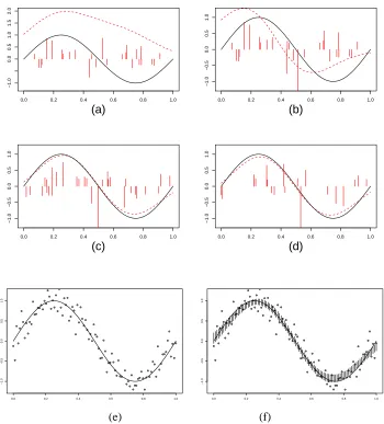
5.1.3 ILLUSTRATION ONSIMULATEDDATA

Data is generated from a noisy sinusoid

f(xi) =sin(2πxi) +εi for x∈[0,1], (19)

(19)

to this data. We setε=0.01 and(pb,pu,pd) = (0.4,0.2,0.4), in algorithms 1 and 2. In Figure 1a-d we plot the target sinusoid, the function realized at an iteration t of the Markov chain, and the jump locations and magnitudes of the random measure. In Figure 1e,f we provide a plot of the target function, realization of the data, and the 95% point-wise credible band—the 95% credible interval at each point xi.

0.0 0.2 0.4 0.6 0.8 1.0

−1.0

0.0

0.5

1.0

1.5

2.0

(a)

0.0 0.2 0.4 0.6 0.8 1.0

−1.0

−0.5

0.0

0.5

1.0

(b)

0.0 0.2 0.4 0.6 0.8 1.0

−1.0

−0.5

0.0

0.5

1.0

(c)

0.0 0.2 0.4 0.6 0.8 1.0

−1.0

−0.5

0.0

0.5

1.0

(d)

0.0 0.2 0.4 0.6 0.8 1.0

−1.0

−0.5

0.0

0.5

1.0

0.0 0.2 0.4 0.6 0.8 1.0

−1.0

−0.5

0.0

0.5

1.0

(e) (f)

(20)

5.2 Classification of Gene Expression Data

For Dirichlet processes there is extensive literature on exact posterior inference using MCMC meth-ods (West, 1992; Escobar and West, 1995; MacEachern and M ¨uller, 1998; M ¨uller et al., 2004) as well as work on approximate inference using variational methods (Blei and Jordan, 2006). Recently Dirichlet process priors have been applied to a Bayesian kernel model for high dimensional data. For example in Liang et al. (2006) and Liang et al. (2007) the Bayesian kernel model was used to classify gene expression data as well as digits, the MNIST database. We apply this model to gene expression data consisting of microarray gene expression profiles from 190 cancer samples and 90 normal samples (Ramaswamy et al., 2001; Mukherjee et al., 2003), over 16,000 genes.

The model is based upon the integral operator given in Equation (17)

f(x) =

Z

XK(x,u)Z(du) =

Z

Xw(u)K(x,u)F(du),

where the random signed measure Z(du)is modeled by a random probability distribution function

F(du)and a random weight function w(u). We assume that the support of Z(du) and w(u)F(du) are equal. A key point in our model will be that if our estimate of F is discrete and puts masses wi at support points (or “knots”) ui, then the expression for f(·)is simply

f(x) =

∑

i

w(ui)K(x,ui).

The above model, in which basis functions are placed at random locations and a joint distribution is specified for the coefficients, has been considered previously in the literature (see Neal, R. M. 1996 and Liang et al. 2007). In Liang et al. (2007) uncertainty about F is expressed using a Dirichlet process prior, Dir(α,F0). The posterior after marginalization is also a Dirichlet distribution and given data(x1, . . . ,xn)the posterior will have the following representation (Liang et al., 2007, 2006)

ˆ

f(x) = α

α+n

Z

w(u)K(x,u)F0(du) + 1

α+n n

∑

i=1

w(xi)K(x,xi),

which can be approximated by the following discrete summation

ˆ f(x)_≈

n

∑

i=1

wiK(x,xi) (20)

when α_n is small and wi=w_α(₊xi_n). We specify a mixture-normal prior on the coefficients wias in Liang et al. (2007) and use the same MCMC algorithm to simulate the posterior.

Note that although Equation (20) has the same form as the representer theorem, it is derived from a very different formulation. In fact, when there is unlabeled data available—(xn+1, . . . ,xn+m)

drawn from the marginρX—our model has the following discrete representation

ˆ f(x) =

n

∑

i=1

wiK(x,xi) + m

∑

i=1

wi+nK(x,xi+n),

where w`=_αw₊(_mx`₊)_n. The above form is identical to the one obtained via the manifold regularization

(21)

perspectives. This simple incorporation of unlabeled data into the model further illustrates the advantage of placing the prior over random measures in the Bayesian kernel model.

In our experiments we first applied a standard variation filter to reduce the number of genes to

p=2800. We then randomly assigned 20% of the samples from the cancer and normal groups to

training data and use the remaining 80% as test data. We used a linear kernel in the model and we used the classification model detailed in Liang et al. (2007).

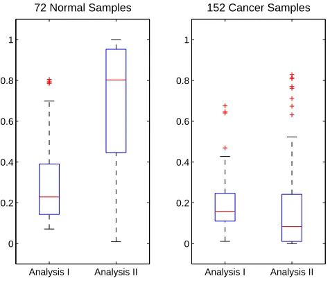
We performed two analyses on this data:

Analysis I—The training data were used in the model and the posterior probability was sim-ulated for each point in the test set. A linear kernel was used.

Analysis II—The training and unlabeled test data were used in the model and the posterior probability was simulated for each point in the test set. A linear kernel was used.

The classification accuracy for Analyses I and II were 73% and 85%, respectively. The accuracy of the predictive models in Analysis I is comparable to that obtained for support vector machines in Mukherjee et al. (2003). Figure 2 displays boxplots of the posterior mean of the 72 the normal and 152 cancer samples for the two analyses.

Analysis I Analysis II 0

0.2 0.4 0.6 0.8 1

72 Normal Samples

Analysis I Analysis II 0

0.2 0.4 0.6 0.8 1

152 Cancer Samples

(22)

6. Discussion

The modeling objective underlying this paper is to formulate a coherent Bayesian perspective for regression using a RHKS model. This requires a firm theoretical foundation characterizing the function space that the Bayesian kernel model spans and the relation of this space to the RKHS. Our results in Section 2 are interesting in their own right, in addition to providing this foundation.

We examined the function class defined by the Bayesian kernel model, the integral of a kernel with respect to a signed Borel measure

G

=

f

f(x) =

Z

XK(x,u)γ(du), γ∈Γ

,

whereΓ_⊆B₍

X

_{). We stated an equivalence under certain conditions of the function class}

G

_and

the RKHS induced by the kernel. This implies: (a) a theoretical foundation for the use of Gaus-sian processes, Dirichlet processes, and other jump processes for non-parametric BayeGaus-sian kernel models, (b) an equivalence between regularization approaches and the Bayesian kernel approach, and (c) an illustration of why placing a prior on the distribution is natural approach in Bayesian non-parametric modelling.

Coherent non-parametric methods have been of great interest in the Bayesian community, how-ever function analytic issues have not been considered. Conversely theoretical studies of RKHS have not approached the approximation and estimation problems from a Bayesian perspective (the exception to both of these are the works of Wahba 1990 and Diaconis 1988). It is our view that the interface of these perspectives is a promising area of research for statisticians, computer scientists, and mathematicians and has both theoretical and practical implications.

A better understanding of this interface may lead to a better understanding of the following research problems:

1. Posterior consistency: It is natural to expect the posterior distribution to concentrate around the true function since the posterior distribution is a probability measure on the RKHS. A natural idea is to use the equivalence between the RKHS and our Bayesian model to exploit the well understood theory of RKHS in proving posterior consistency of the Bayesian ker-nel model. Tools such as concentration inequalities, uniform Glivenko-Cantelli classes, and uniform central limit theorems may be helpful.

2. Priors on function spaces: In this paper we discuss general function classes without concern for more subtle smoothness properties. An obvious question is can we use the same ideas to relate priors on measures and the kernel to specific classes of functions, such as Sobolev spaces. A study of the relation between integral operators and priors could lead to interesting and useful results for putting priors over specific function classes using the kernel model.

3. Comparison of process priors for modeling: A theoretical and empirical comparison of the accuracy of the various process priors on a variety of function classes and data sets would be of great practical importance and interest, especially for high dimensional problems.

(23)

known (Bousquet and Elisseeff, 2002; Poggio et al., 2004). Further developing this relation is a very interesting area of research and may be of importance for the posterior consistency of the Bayesian kernel model.

Acknowledgments

We would like to thank the reviewers for many useful suggestions and comments. FL would like to acknowledge NSF grant DMS 0406115. SM and QW would like to acknowledge support for this project from the Institute for Genome Sciences & Policy at Duke as well as the NIH grant P50 HG 03391-02 for the Center for Public Genomics. RW would like to acknowledge NSF grants DMS–0112069 and DMS–0422400. Any opinions, findings, and conclusions or recommendations expressed in this material are those of the authors and do not necessarily reflect the views of the National Science Foundation.

Appendix A. Proofs of Propositions

In this appendix we provide proofs for the propositions in Section 2.

A.1 Proof for Proposition 4 It holds that

kL_K_[γ_]_k2_Kk₌_k

∑

j∈Λ

λjajφjk2K=

∑

j∈Λ

(λjaj)2

λj

=

∑

j∈Λ

λja2j

which is upper bounded byλ1∑ja2j <∞. HenceLK[γ]∈

H

K. By direct computation, we have hL_K_[γ_]_,γ_i₂₌

∑

λjakφj,

∑

ajφj

2=

∑

λka 2

j =kLK[γ]k2K. A.2 Proof for Corollary 5

The first claim is obvious since bothL_K_[L2₍

X

_,_du)]_and

H

K are the same finite dimensional space

spanned byφ

j _j_∈_Λ.

The second claim follows from the existence of the sequence(cj)j∈Λsuch that

∑

j∈Λ c2_j

λj

<∞ and

∑

j∈Λ

c2_j

λ2 j

=∞.

For any such sequence, the function f =∑j∈Λcjφj lies in

H

K. But by Proposition 4, one cannot find aγ_∈L2(

X

,du)such thatL_K_[γ_{] =} _{f . A simple example is}_(c_j₎_j

∈Λ= (λj)j∈Λ.

If K is strictly positive definite, then all its eigenvalues are positive. So the last claim holds.

A.3 Proof for Proposition 6

(24)

{γn}n_≥1⊂L2(

X

,du)which converges toγin L1(

X

,du). It follows from Proposition 4 thatLK[γn]∈

H

K and

kL_K_[γ_n_]_k2

K=

Z

X

Z

XK(u,v)γn(u)duγn(v)dv≤κ 2Z

X|γn(u)|du

Z

X|γn(v)|dv=κ 2

kγnk21<∞. Therefore we have_{L_K_[γ_n_]_}n

≥1⊂

H

K and lim

n_→∞_msup_>_nk

L_K_[γ_n_]₋L_K_[γ_m_]_kK_≤ _lim

n_→∞_msup_>_nκkγn−γmk1=0, so_{L_K_[γ_n_]_}n

≥1is a Cauchy sequence in

H

K. By completeness it converges to some f ∈

H

K. The

proof will be finished if we showL_K_[γ_{] =} _{f .}

By the reproducing property of

H

K convergence in the RKHS norm implies point-wise

conver-gence for x_∈

X

, so LK[γn](x)→ f(x)for every x. In addition, for every x_∈

X

,we have

lim n→∞|

L_K_[γ_n_](x)₋L_K_[γ_](x)_{| ≤}

Z

X|K(x,u)(γn(u)−γ(u))|du≤κ 2

kγn−γk1=0, which implies thatL_K_[γ_n_](x)_{also converges to}L_K_[γ_{](x). Hence}L_K_[γ_{] =} _f _∈

H

_K_.

Letγ=∑ciδxi∈MD. ThenLK[γ] =∑ciKxi and

kL_K_[γ_]_k2

K=

∑

i,j

ciK(xi,xj)cj≤κ2

∑

i

|ci|

!2

<∞.

Therefore, our conclusion holds.

The arguments for Lebesgue measure hold if we replace the Lebesgue measure with any finite Borel

measure. We denote the corresponding integral operator asL_K_,_µ _{and function space of integrable}

and square integrable functions as L1_µ(

X

)and L2_µ(

X

)respectively. Then L2_µ(

X

)_⊂L1_µ(

X

)_⊂L−_K1_,_µ(

H

K). Since the function 1X(x) =1 lies in L_µ1(

X

)we obtain

L_K_{(µ) =}L_K_,_µ₍₁_X_{) =}

Z

XK(·,u)dµ(u)∈

H

K. This impliesB₊₍

X

₎_{lies in L}−1

K (

H

K)and so doesB(

X

).

Appendix B. Multivariate Version of L´evy-Khintchine Formula