Quasi-Geodesic Neural Learning Algorithms Over
the Orthogonal Group: A Tutorial
Simone Fiori [email protected]
Facolt`a di Ingegneria, Universit`a di Perugia Polo Didattico e Scientifico del Ternano Localit`a Pentima bassa, 21, I-05100 Terni, Italy
Editor: Yoshua Bengio
Abstract
The aim of this contribution is to present a tutorial on learning algorithms for a single neural layer whose connection matrix belongs to the orthogonal group. The algorithms exploit geodesics appro-priately connected as piece-wise approximate integrals of the exact differential learning equation. The considered learning equations essentially arise from the Riemannian-gradient-based optimiza-tion theory with deterministic and diffusion-type gradient. The paper aims specifically at reviewing the relevant mathematics (and at presenting it in as much transparent way as possible in order to make it accessible to readers that do not possess a background in differential geometry), at bring-ing together modern optimization methods on manifolds and at comparbring-ing the different algorithms on a common machine learning problem. As a numerical case-study, we consider an application to non-negative independent component analysis, although it should be recognized that Rieman-nian gradient methods give rise to general-purpose algorithms, by no means limited to ICA-related applications.
Keywords: differential geometry, diffusion-type gradient, Lie groups, non-negative independent
component analysis, Riemannian gradient
1. Introduction
From the scientific literature, it is known that a class of learning algorithms for artificial neural networks may be formulated in terms of matrix-type differential equations of network’s learnable parameters, which give rise to learning flows on parameters’ set. Often, such differential equations are defined over parameter spaces that may be endowed with a specific geometry, such as the general linear group, the compact Stiefel manifold, the orthogonal group, the Grassman manifold and the manifold of FIR filters1 (Amari, 1998; Fiori, 2001, 2002; Liu et al., 2004; Zhang et al., 2002), that describes the constraints that the network parameters should fulfill and that is worth taking into account properly. From a practical viewpoint, the mentioned differential equations should be integrated (solved) properly through an appropriate numerical integration method that allows us to preserve the underlying structure (up to reasonable precision). This may be viewed as defining a suitable discretization method in the time domain that allows converting a differential learning equation into a discrete-time algorithm.
With the present contribution, we aim at studying and illustrating learning algorithms for a single neural layer whose connection matrix belongs to the orthogonal group, that is the group of square orthogonal matrices. As an appropriate approximation of the exact learning flows, the algorithms exploit approximate geodesics suitably glued together, as formerly proposed by Fiori (2002) and Nishimori (1999).
As a case-study, we consider an application to geodesic-learning-based non-negative indepen-dent component analysis, as proposed by Plumbley (2003). We present three different learning algorithms that are based on gradient-type optimization of a non-negative independent component analysis criterion over the group of orthogonal matrices. The first two algorithms arise from the direct application of Riemannian gradient optimization without and with geodesic line search, as proposed by Plumbley (2003). The third algorithm relies on a randomized gradient optimization based on diffusion-type Riemannian gradient, as proposed by Liu et al. (2004).
The contribution of the present tutorial may be summarized via the following key points:
• It provides a clear and well-motivated introduction to the mathematics needed to present the geometry-based learning algorithms.
• It clearly states and illustrates the idea that, when we wish to implement a gradient-based algorithm on a computer, it is necessary to discretize the differential learning equations in some suitable way (the ‘gradient flow’ simply cannot be computed exactly in practice).
• In order to effect such discretization, we may not employ standard discretization methods (such as the ones based on Euler forward-backward discretization), that do not work as they stand on curved manifolds. We should therefore resort to more sophisticated integration tech-niques such as the one based on geodesics.
• In order to improve the numerical performances of the learning algorithm, we might ten-tatively try adding some stochasticity to the standard gradient (through annealed-MCMC method) and try a geodesic search. It is not guaranteed that the above-mentioned improve-ment works on a concrete application, therefore it is worth testing them on ICA+ problem. The results on this sides are so far disappointing, because numerical simulations shown that standard Riemannian gradient with no geodesic search nor stochasticity added outperforms the other methods on the considered ICA+problem.
Although in the machine learning community the presented differential geometry-based learn-ing algorithms have so far been primarily invoked in narrow contexts such as principal/independent component analysis (interested readers might want to consult, for example, Fiori (2001), Celledoni and Fiori (2004) and Plumbley (2003) for a wide review), it should be recognized that differential-geometrical methods provide a general-purpose way of designing learning algorithms, which is profitable in those cases where a learning problem may be formulated mathematically as an opti-mization problem over a smooth manifold. Some recent advances and applications of these methods are going to be described in the journal special issue whose content is summarized in the editorial by Fiori and Amari (2005).
curves. Then, these results are customized to the case of the orthogonal group of concern in the present paper. Geodesic-based approximations of gradient-type learning differential equations over the orthogonal group are also explained. The Section 2 also presents some notes on the stability of such learning equations as well as on the relationship between the presented learning theory and the well-known natural-gradient theory and information geometry theory. Section 3 presents two deterministic-gradient learning algorithms, one of which is based on the optimization of the learning stepsize via ‘geodesic search’. Next, the concept of diffusion-type gradient on manifolds is recalled in details and a third learning algorithm based on it is presented. Such learning algorithm also takes advantage of simulated annealing optimization technique combined with Markov-Chain Monte-Carlo sampling method, which are also recalled in the Section 3, along with some of their salient features. Section 4 deals with non-negative independent component analysis. Its definition and main properties are recalled and the orthogonal-group Riemannian-gradient of the associated cost function is computed. Such computation allows customizing the three generic Riemannian-gradient-based geodesic algorithms to the non-negative independent component analysis case. Also, a fourth projection-based algorithm is presented for numerical comparison purpose. The details of algorithms implementation and the results of computer-based experiments performed on non-negative independent component analysis of gray-level image mixtures are also illustrated in the Section 4. Section 5 concludes the paper.
2. Learning Over the Orthogonal Group: Gradient-Based Differential Systems and Their Integration
The aims of the present section are to recall some basic concepts from differential geometry and to derive the general form of gradient-based learning differential equations over the orthogonal group. We also discuss the fundamental issue of solving numerically such learning differential equations in order to obtain a suitable learning algorithm.
2.1 Basic Differential Geometry Preliminaries
In order to better explain the subsequent issues, it would be beneficial to recall some basic concepts from differential geometry related to the orthogonal group O(p).
An algebraic group(G,m,i,e)is a set G that is endowed with an internal operation m : G×G→ G, usually referred to as group multiplication, an inverse operation i : G→ G, and an identity element e with respect to the group multiplication. These objects are related in the following way. For every elements x,y,z∈G, it holds that
m(x,i(x)) =m(i(x),x) =e,m(x,e) =m(e,x) =x and m(x,m(y,z)) =m(m(x,y),z).
Note that, in general, the group multiplication is not commutative, that is, given two elements x,y∈G, it holds m(x,y)6=m(y,x).
Two examples of algebraic groups are(ZZ,+,−,0)and(Gl(p),·,−1,I
p). The first group is the
set of all integer numbers endowed with the standard addition as group multiplication. In this case, the inverse is the subtraction operation and the identity is the null element. In the second example, we considered the set of non-singular matrices:
endowed with standard matrix multiplication ‘·’ as group multiplication operation. In this case, the inverse is the standard matrix inverse and the identity is the identity matrix Ip. It is easy to show
that both groups operations/identity satisfy the above general conditions. As a counterexample, the set of the non-negative integer numbers ZZ+0(≡IN) does not form a group under standard ad-dition/subtraction. A remarkable difference between the two groups above is that the first one is a discrete group while the second one is a continuous group.
A useful concept for the economy of the paper is the one of differential manifold. The formal definition of a differential manifold is quite involved, because it requires precise definitions from mathematical topology theory and advanced calculus (Olver, 2003). More practically, a manifold may be essentially regarded as a generalization of curves and surfaces in high-dimensional space, that is endowed with the noticeable property of being locally similar to a flat (Euclidean) space. Let us consider a differential manifold
M
and a pointξon it. From an abstract point of view,ξis an element of a setM
and does not necessarily possess any particular numerical feature. In order to be able to make computations on manifolds, it is convenient to ‘coordinatize’ it. To this aim, a neighborhood (open set) U⊂M
is considered, whichξbelongs to, and a coordinate mapψ: U→E
is defined, whereE
denotes a Euclidean space (as for example, IRp– the set of p-dimensional real-valued vectors – or IRp×p – the set of the p×p real-valued matrices –). The function ψneeds to be a one-to-one map (homeomorphism). In this way, we attach a coordinate x=ψ(ξ)to the pointξ. Asψis a homeomorphism, there is a one-to-one correspondence between a point on a manifold and its corresponding coordinate-point, therefore normally the two concepts may be confused and we may safely speak of a point x∈
M
. About these concepts, two short notes are in order:• Borrowing terms from maritime terminology, a triple (ψ,U,p) is termed coordinate chart associated to the manifold
M
. Such notation evidences that the elementsψand U⊂M
are necessary to coordinatize a point on the manifold and that the coordinate space has dimension p. If the dimension is clear from the context, the indication of p may of course be dispensed of.• A main concept of differential geometry is that every geometrical property is independent of the choice of the coordinate system. As a safety note, it is important to remark that, when we choose to express geometrical relationships in coordinates (as it is implicitly assumed by the above-mentioned ‘confusion’ between a pointξ∈
M
and its coordinate x∈E
) we are by no means abandoning this fundamental principle, but we are obeying to the practical need of algorithm implementation on a computer that requires – of necessity – some explicit representation of the quantities of interest.In general, it is impossible to cover a whole manifold with a unique coordinate map. Therefore, the procedure for coordinatizing a manifold generally consists in covering it with a convenient number of neighborhoods Uk, each of which is endowed with a coordinate map ψk : Uk →
E
k,with
E
k being an Euclidean space of dimension p, which, by definition, denotes the dimension of the manifold itself. Technically, the set {Uk} is termed a basis for the manifold and it doesnot need to be finite (but it is inherently countable). It is important to note that, in general, the neighborhoods Uk may be overlapping. In this case, the mapsψk need to satisfy some constraints
represent coordinate changes, should be diffeomorphisms, that is, C∞functions endowed with C∞ inverse.
A smooth manifold is by nature a continuous object. A simple example is the unit hyper-sphere Spdef={x∈IRp+1|xTx=1}. This is a smooth manifold of dimension p embedded in the Euclidean space IRp+1, in fact with only p coordinates we can identify any point on the sphere. Olver (2003) shows how to coordinatize such manifold through for example, the stereographic projection, which requires two coordinate maps applied to two convenient neighborhoods on the sphere.
An interesting object we may think to on a differential manifold
M
is a smooth curveγ:[a,b]→M
. In coordinates,2x=γ(t)describes a curve on the manifoldM
delimited by the endpointsγ(a) andγ(b). Here, the manifold is supposed to be immersed in a suitable ambient Euclidean spaceA
of suitable dimension (for instance, the sphere Sp may be though of as immersed in the ambient spaceA
=IRp+1).Let us now suppose 0∈[a,b]and let us consider a curveγpassing by a given point x∈
M
, namely x=γ(0). The smooth curve admits a tangent vector vxat the point x on the manifold, whichis defined by
vx
def =lim
t→0
γ(t)−γ(0)
t ∈
A
.Clearly, the vector vx does not belong to the curved manifold
M
but is tangent to it in the pointx. Let us imagine to consider every possible smooth curve on a manifold of dimension p passing through the point x and to compute the tangent vectors to these curves in the point x. The collection of these vectors span a linear space of dimension p, which is referred to as tangent space to the manifold
M
at the point x, and is denoted with TxM
⊆A
.As a further safety note, it might deserve to recall that, in differential geometry, the main way to regard for example, tangent spaces and vector fields is based on differential operators (Olver, 2003). This means, for instance, that a tangent vector v∈Tx
M
of some smooth manifoldM
isdefined in such a way that if
F
denotes a smooth functional space then for instance v :F
→IR, namely v(f)is a scalar for f ∈F
. In this paper we chose not to invoke such notation. The reason is that we are interested in a special matrix-type Lie group (the orthogonal group), whose geometry may be conveniently expressed in terms of matrix-type quantities/operations. The theoretical bridge between the differential-operator-based representation and the matrix-based representation is given by the observation that every differential operator in TxM
may be written as a linear combination ofelementary differential operators, that form a basis for the tangent space, through some coefficients. The structure of the tangent space is entirely revealed by the relationships among these coefficients. Therefore, we may choose to represent tangent vectors as algebraic vectors/matrices of coefficients, that is exactly what is implicitly done here.
It is now possible to give the definition of Riemannian manifold, which is a pair(
M
,g)formed by a differential manifoldM
and an inner product gx(vx,ux), locally defined in every point x ofthe manifold as a bilinear function from Tx
M
×TxM
to IR. It is important to remark that the innerproduct gx(·,·) acts on elements from the tangent space to the manifold at some given point, it
therefore depends (smoothly) on the point x.
On a Riemannian manifold(
M
,g), we can measure the length of a vector v∈TxM
askvkdef=pgx(v,v).
Also, a remarkable property of Riemannian manifolds is that we can measure the length of a curve
γ:[a,b]→
M
on the manifold through the local metric on its tangent spaces. In fact, the length of the curveγ(·)is, by definition, Lγdef=Rabds, where ds is the infinitesimal arc length. From geometrywe know that ds=kγ˙(t)kdt, therefore we have
Lγ=
Z b
a
q
gγ(t)(˙γ(t),˙γ(t))dt. (2)
The net result of this argument is that, through a definition of an inner product on the tangent spaces to a Riemannian manifold, we are able to measure the length of paths in the manifold itself, and this turns the manifold into a metric space.
A vector field vx on manifold
M
specifies a vector belonging to the tangent space TxM
to themanifold at every point x.
With the notions of vector field and curve on a manifold, we may define the important concept of geodesics. A geodesic on a smooth manifold may be intuitively looked upon in at least three different ways:
• On a general manifold, the concept of geodesic extends the concept of straight line on a flat space to a curved space. An informal interpretation of this property is that a geodesic is a curve on a manifold that would resemble a straight line in an infinitesimal neighborhood of any of its points. The formal counterpart of this interpretation is rather involved because it requires the notion of covariant derivative of a vector field with respect to another vector field and leads to a second-order differential equation involving the Christoffel structural functions of the manifold (Amari, 1989).
• On a Riemannian manifold, a geodesic among two points is locally defined as the shortest curve on the manifold connecting these endpoints. Therefore, once a metric g(·,·)is specified, the equation of the geodesic arises from the minimization of the functional (2) with respect to
γ. In general, the obtained equation is difficult to solve in closed form.
• Another intuitive interpretation is based on the observation that a geodesic emanating from a point x on the manifold coincides to the path followed by a particle sliding on the manifold itself with constant scalar speed specified by the norm of the vector vx. For a manifold
em-bedded in a Euclidean space, this is equivalent to require that the acceleration of the particle is either zero or perpendicular to the tangent space to the manifold in every point.
The concept of geodesic and geodesic equation are recalled here only informally. Appendix A provides a detailed account of these and related concepts just touched here, such as the Christoffel functions (or affine-connection coefficients).
An important vector field often considered in the literature of function optimization over man-ifolds is the gradient vector field. If we consider a smooth function f :
M
→IR and define its gradient gradMx f , then a oft-considered differential equation is:dx
dt =±grad
M
x f, (3)
Formally, the concept of gradient on a Riemannian manifold may be defined as follows. Let us consider a Riemannian manifold(
M
,g)and, for every point x, the tangent space TxM
. Let us alsoconsider a smooth function f :
M
→IR, the standard Euclidean inner product gE in TxM
and theJacobian gradEx f =∂∂xf of the function f with respect to x. The Riemannian gradient gradMx f of the function f over the manifold
M
in the point x is uniquely defined by the following two conditions:• Tangency condition. For every x∈
M
, gradMx f∈TxM
.• Compatibility condition. For every x∈
M
and every v∈TxM
, gx(gradMx f,v) =gE(gradE
x f,v).
The tangency condition expresses the fact that a gradient vector is always tangent to the base-manifold, while the compatibility condition states that the inner product, under a metric on a mani-fold, of a gradient vector with any other tangent vector is invariant with the chosen metric. However, note that the gradient does depend on the metric. The ‘reference’ inner product is assumed as the Euclidean inner product that a flat space may be endowed with. For instance, if the base manifold
M
has dimension p, then it may be assumedE
=TxE
=IRpin every point x and gE(u,v) =vTu.It is worth noting that such special metric is uniform, in that it does not actually depend on the point x.
In order to facilitate the use of the compatibility condition for gradient computation, it is some-times useful to introduce the concept of normal space of a Riemannian manifold in a given point under a chosen metric gA:
Nx
M
def
={n∈
A
|gAx(n,v) =0, ∀v∈TxM
}.It represents the orthogonal complement of the tangent space with respect to an Euclidean ambient space
A
that the manifoldM
is embedded within.With the notion of algebraic group and smooth manifold, we may now define a well-known object of differential geometry, that is the Lie group. A Lie group conjugates the properties of an algebraic group and of a smooth manifold, as it is a set endowed with both group properties and manifold structure. An example of a Lie group that we are interested in within the paper is the orthogonal group:
O(p)def={X∈IRp×p|XTX=Ip}. (4)
It is easy to verify that it is a group (under standard matrix multiplication and inversion) and it is also endowed with the structure of a smooth manifold.
Consequently, we may for instance consider the tangent space TxG of a Lie group G at the point
x. A particular tangent space is TeG, namely the tangent at identity, which, properly endowed with
a binary operator termed Lie bracket, has the structure of a Lie algebra and is denoted withg. An essential peculiarity of the Lie groups (G,m,i,e) is that the whole group may be always brought back to a convenient neighborhood of the identity e and the same holds for every tangent space TxG,∀x∈G, that may be brought back to the algebrag. Let us consider, for instance, a curve
γ(t)∈G passing through the point x, with t∈[a,b]such that 0∈[a,b]and x=γ(0). We may define the new curve ˜γ(t)def=m(γ(t),i(x))that enjoys the property ˜γ(0) =e; conversely, γ(t) =m(˜γ(t),x). This operation closely resembles a translation of a curve into a convenient neighborhood of the group identity, so that we can define a special operator referred to as right translation as
Rx: G→G,Rx(γ)
def
It is clear that every tangent vector vxto the curve γat x is also translated to a tangent vector ˜v of
the curve ˜γ(t)by a conveniently defined operator:
dRx: TxG→TeG,˜v=dRx(v),
which is commonly referred to as tangent map associated to the (right) translation Rx. Such map
is invertible and allows us to translate a vector belonging to a tangent space of a group to a vector belonging to its algebra (and vice-versa).3
From the above discussion, it is straightforward to see that, if the structure of gis known for a group G, it might be convenient to coordinatize a neighborhood of the identity of G through elements of the associated algebra with the help of a conveniently-selected homeomorphism. Such homeomorphism is known in the literature as exponential map and is denoted with exp :g→G. It is important to recall that ‘exp’ is only a symbol and, even for matrix-type Lie groups, does not necessarily denote matrix exponentiation.
2.2 Gradient Flows on the Orthogonal Group
As mentioned, the orthogonal group O(p)is a Lie group, therefore it is endowed with a manifold structure. Consequently, we may use the above-recalled instruments in order to define gradient-based learning equations of the kind (3) over O(p)and to approximately solve them.
Some useful facts about the geometrical structure of the orthogonal group O(p)are:
• The standard group multiplication on O(p)is non-commutative (for p≥3).
• The group O(p) manifold structure has dimension p(p2−1). In fact, every matrix in O(p) possesses p2entries which are constrained by p(p2+1) orthogonality/normality restrictions. • The inverse operation i(X) =X−1coincides with the transposition, namely i(X) =XT. • The tangent space of the Lie group O(p) has the structure TXO(p) ={V∈IRp×p|VTX+
XTV=0p}. This may be proven by differentiating a generic curve γ(t) ∈O(p) passing
by X for t=0. Every such curve satisfies the orthogonal-group characteristic equation (4), namelyγT(t)γ(t) =Ip, therefore, after differentiation, we get ˙γT(0)γ(0) +γT(0)˙γ(0) =0p. By
recalling that the tangent space is formed by the velocity vectors ˙γ(0), the above-mentioned result is readily achieved.
• The Lie algebra associated to the orthogonal group is the set of skew-symmetric matrices so(p)def={V˜ ∈IRp×p|V˜ +V˜T=0
p}. In fact, at the identity(X=Ip), we have TIpO(p) =so(p).
• The Lie algebraso(p)is a vector space of dimension p(p2−1).
First, it is necessary to compute the gradient of a function f : O(p)→IR over the group O(p)in view of computing the geodesic that emanates from a point X∈O(p)with velocity proportional to gradOX(p)f . In this derivation, we essentially follow the definition of Riemannian gradient given in Section 2.1.
Let the manifold O(p)be equipped with the canonical induced metric gO(p), that is gXO(p)(U,V)def= tr[UTV], for every X∈O(p)and every U,V∈T
XO(p). This metric coincides with the standard
Eu-clidean metric gIRp×p in IRp×p. Having endowed the manifold O(p)with a metric, it is possible to describe completely its normal space, provided the ambient space
A
is endowed with the canonical Euclidean metric. In fact, we haveNXO(p) ={N=XS∈IRp×p|tr[NTV] =0, ∀V∈TXO(p)}.
The matrix S should have a particular structure. In fact, the normality condition, in this case, writes 0=tr[VT(XS)] =tr[SVTX] =tr[(XTV)ST]. The latter expression, thanks to the structure of tan-gent vectors, is equivalent to−tr[(VTX)ST], therefore the normality condition may be equivalently rewritten as tr[(VTX)(S−ST)] =0. In order for this to be true, in the general case, it is necessary and sufficient that S=ST. Thus:
NXO(p) ={XS|ST=S∈IRp×p}.
Let gradOX(p)f be the gradient vector of f at X∈O(p)derived from the metric gO(p). According to the compatibility condition for the Riemannian gradient:
gIRXp×p(V,gradIRXp×pf) =gOX(p)(V,gradOX(p)f),
for every tangent vector V∈TXO(p), therefore:
gXIRp×p(V,gradXIRp×pf−gradOX(p)f) =0,
for all V∈TXO(p). This implies that the quantity gradIR
p×p
X f−grad
O(p)
X f belongs to NXO(p).
Explicitly:
gradXIRp×pf=gradXO(p)f+XS. (5) In order to determine the symmetric matrix S, we may exploit the tangency condition on the Rie-mannian gradient, namely(gradOX(p)f)TX+XT(gradO(p)
X f) =0p. Let us first pre-multiply both sides
of the equation (5) by XT, which gives
XTgradIRXp×pf=XTgradOX(p)f+S.
The above equation, transposed hand-by-hand, becomes
(gradXIRp×pf)TX= (gradXO(p)f)TX+S.
Hand-by-hand summation of the last two equations gives
(gradIRXp×pf)TX+XT(gradIRXp×pf) =2S,
that is:
S=(grad IRp×p
X f)TX+XT(gradIR
p×p
X f)
2 . (6)
By plugging the expression (6) into expression (5), we get the form of the Riemannian gradient in the orthogonal group, which is:
gradOX(p)f= grad IRp×p
X f−X(gradIR
p×p
X f)TX
About the expression of the geodesic, as mentioned, in general it is not easy to obtain in closed form. In the present case, with the assumptions considered, the geodesic on O(p)departing from the identity with velocity ˜V∈so(p)has expression ˜γ(t) =exp(t ˜V). (It is immediate to verify that ˜
γ(0) =Ip and d ˜γdt(t)
t=0= ˜
V.) It might be useful to verify such essential result by the help of the
following arguments.
As already recalled in Section 2.1, when a manifold is embedded in a Euclidean space, the second derivative of the geodesic with resepct to the parameter is either zero or perpendicular to the tangent space to the manifold in every point (see Appendix A). Therefore, a geodesic ˜γ(t) on the Riemannian manifold(O(p),gO(p)) embedded in the Euclidean ambient space(IRp×p,gIRp×p
), departing from the identity Ip, should be such that ¨˜γ(t)∈NIpO(p), therefore it should hold:
¨˜
γ(t) =˜γ(t)S(t),with ST(t) =S(t). (7)
Also, we known that any geodesic branch belongs entirely to the base manifold, therefore ˜γT(t)˜γ(t) =
Ip. By differentiating two times such expression with respect to the parameter t it is easily gotten:
¨˜
γT
(t)˜γ(t) +2˙˜γT(t)˙˜γ(t) +γ˜T(t)¨˜γ(t) =0p. (8)
By plugging equation (7) into equation (8), we find S(t) =−γ˙˜T(t)˙˜γ(t), which leads to the second-order differential equation on the orthogonal group:
¨˜
γ(t) =−˜γ(t)(˙˜γT(t)˙˜γ(t)),
to be solved with initial conditions ˜γ(0) =Ipand ˙˜γ(0) =V. It is a straightforward task to verify that˜
the solution to this second-order differential equation is given by the one-parameter curve ˜γ(t) = exp(t ˜V), where exp(·)denotes matrix exponentiation.
The expression of the geodesic in the position of interest may be made explicit by taking advan-tage of the Lie-group structure of the orthogonal group endowed with the canonical metric. In fact, let us consider the pair X∈O(p)and gradOX(p)f∈TXO(p)as well as the geodesicγ(t)that emanates
from X with velocity V proportional to gradOX(p)f , and let us suppose for simplicity thatγ(0) =X.
Let us now consider the right-translated curve ˜γ(t) =γ(t)XT. The new curve enjoys the following
properties:
1. It is such that ˜γ(0) =Ip, therefore it passes through the identity of the group O(p).
2. The tangent vector V to the curve at X is ‘transported’ into the tangent vector:
˜
V=VXT, (9)
at the identity, so ˜V∈so(p).
3. As the right-translation is an isometry, the curve ˜γ(t) is still a geodesic departing from the identity matrix with velocity proportional to ˜V= (gradOX(p)f)XT.
From these observations, we readily obtain the geodesic in the position of interest X∈O(p), namely
γ(t) =exp(t ˜V)X.
As this is an issue of prime importance, we deem it appropriate to verify that the curveγ(t)just defined belongs to the orthogonal group at any time. This may be proven by computing the quantity
γT(t)γ(t)and taking into account the identity expT(t ˜V) =exp(−t ˜V). Then we have
γT(t)γ(t) =XTexpT(t ˜V)exp(t ˜V)X=XTexp(
2.3 Comments on Stability and the Relationship with Natural Gradient Theory
Some comments on the questions of the stability of gradient-based learning algorithms on the or-thogonal group and on the relationship of Riemannian gradient-based learning algorithms on the orthogonal group with the well-known ‘natural’ gradient-based optimization theory are in order.
When applied to the manifold
M
=O(p), the general gradient-based learning equation (3) has the inherent property of keeping the connection matrix X within the group O(p)at any time. It is very important to note that the discrete-time version of this learning equation, described in Section 3, also enjoys this noticeable property. When for example, learning algorithms based on the manifold Gl(p), defined in equation (1), are dealt with, one of the theoretical efforts required to prove their stability consists in showing that there exists a compact sub-manifold that is an attractor for the learning system. The above observations reveal that the problem of the existence of an orthogonal-group-attractor for discrete-time learning systems based on the orthogonal Lie group does not arise when a proper integration algorithm is exploited. Moreover, as opposed to the Euclidean space IRp and the general-linear group Gl(p), the orthogonal group O(p) is a compact space. This means that no diverging trajectories exist for the learning system (3) or its discrete-time counterpart. Such effect may be easily recognized in the two-dimensional (p=2) case, through the parameterizationψ−1:[−π,π[→SO(2):
X=
cosβ −sinβ sinβ cosβ
. (10)
It is worth noting that det(X) =1, while, in general, the determinant of an orthonormal matrix may be either −1 or +1, in fact 1=det(XTX) =det2(X) for X ∈O(p). This means that the above parameterization spans one of the two components of the orthogonal group termed special orthogonal group and denoted by SO(p). (In the above notation, we easily recognize a coordinate chart(ψ,SO(2),1)associated to O(2).) Now, by singling out the columns of the matrix X= [x1x2], we easily see thatkx1k=kx2k=1, which proves the space SO(2)is compact. The same reasoning may be repeated for the remaining component of O(2).
In its general formulation, the widely-known ‘natural gradient’ theory for learning may be sum-marized as follows. The base-manifold for learning is the group of non-singular matrices Gl(p)that is endowed with a metrics based on the Fisher metric tensor which, in turn, derives from a trun-cated expansion of the Kullback-Leibler informational divergence (KLD) (Amari, 1998). The latter choice derives from the possibility – offered by the KLD – to induce a metrics in the abstract space of neural networks having same topology but different connection parameters, which is referred to as neural manifold.
In the independent component analysis case, a special structure was envisaged by Yang and Amari (1997) for the natural gradient by imposing a Riemannian structure on the Lie group of non-singular matrices Gl(p). We believe it could be useful to briefly recall this intuition here by using the language of Lie groups recalled in Section 2.1. First, the tangent space at identity Ip
to Gl(p) is denoted bygl(p), as usual. Such Lie algebra may be endowed with a scalar product gGlI (p)
p (·,·):gl(p)×gl(p)→IR. As there is no reason to weight in a different way the components of the matrices ingl(p), it is assumed gGlI (p)
p ( ˜
U,V˜)def=tr[U˜TV˜]. The question is now how to define the scalar product in a generic tangent space TXGl(p), with X∈Gl(p). Let us consider, to this purpose,
a curveγ(t)∈Gl(p) passing by the point X at t=0, namelyγ(0) =X. This curve may always
in fact, the inverse X−1 surely exists because Gl(p) is the set of all invertible p×p matrices by definition and now ˜γ(0) =Ip. Therefore, if V∈TXGl(p)denotes the tangent vector to the curveγ(t)
at t=0 and ˜V∈gl(p)denotes the tangent vector to the curve ˜γ(t)at t=0, they are related by the corresponding tangent map V→V˜ =X−1V. This observation may be exploited to define an inner product on the tangent spaces of Gl(p)by imposing the Riemannian-structure invariance property:
gGlX(p)(U,V)def=gGlI (p) p (X
−1U,X−1V) =tr[UT(XT)−1X−1V].
Having defined a general (non-uniform) metric in the tangent spaces to Gl(p), we may now compute the Riemannian (natural) gradient on it, by invoking the tangency and compatibility conditions as stated in Section 2.1. Actually, the tangency condition does not provide any constraint in the present case, because every TXGl(p)is ultimately isomorphic to IRp×p. The compatibility condition,
instead, writes, for a smooth function f : Gl(p)→IR:
gXGl(p)(gradXGl(p)f,V) =tr "
∂ f
∂X
T
V
#
, ∀V∈TXGl(p).
This condition implies:
tr "(
(gradGlX(p)f)T(XT)−1X−1−
∂ f
∂X
T)
V
#
=0,∀V∈TXGl(p)
⇒ (gradGlX(p)f)T(XT)−1X−1= ∂
f
∂X
T
⇒ gradGlX(p)f = (XXT)∂f
∂X.
Of course, a different form for the natural gradient may be obtained by choosing the right-translation ˜
γ(t)def=γ(t)X−1 as a basis for invariance, as done for example, by Yang and Amari (1997). The ‘natural gradient’ theory for Gl(p)and the Riemannian-gradient-theory for the group O(p)are thus somewhat unrelated, even if ultimately the ‘natural gradient’ is a Riemannian gradient on the group Gl(p) arising from a specific metric. Some further details on the optimization problem over the general linear group (about for example, using the exponential map on Gl(p)) have been presented by Akuzawa (2001).
Another interesting comparison is with the information-geometry theory for learning.4 In the spirit of information geometry, the natural gradient works on a manifold of parameterized likeli-hood. Now, in two dimensions, the Riemannian geometry of the orthogonal group, defined by the parameterization (10) above, may be clearly related to the information geometry of the binomial dis-tribution defined by the variables r,q such that r+q=1, via the transform r=cos2(β), q=sin2(β). Whether such link exists in any dimension (p≥3) is not known to the author and would be worth investigating in future works. The same holds for the relationship with second order (Newton) method, which is known for the natural gradient (see, for example, Park et al. (2000) and references therein) but whose relationship with general Riemannian gradient theory is to be elucidated.
3. Learning Over the Orthogonal Group: Three Algorithms
In order to numerically integrate a continuous learning differential equation on a manifold, a proper discretization method should be exploited. On a flat space, a possible discretization method is line approximation based on Euler’s or trapezoidal technique (or some more sophisticated techniques such as the Runge-Kutta method). However, if applied to differential equations based on curved manifolds, such ordinary discretization methods produce updating rules that do not satisfy the man-ifold constraints. Following the general differential-geometric knowledge, two possible ways to tackle the problem are:
• The projection method. It consists in projecting the updated value to the manifold after each iteration step. More formally, this method consists in embedding the manifold
M
of interest into a Euclidean space of proper dimensionA
and to discretize the differential equation whose variable is regarded as belonging toA
through any suitable ordinary method. Then, in each iteration, the newly found approximated solution is projected back to the manifold through a suitable projectorΠ:A
→M
. The next iteration starts from the projected putative solution.• The geodesic method. The principle behind the geodesic method is to replace the line approx-imation to the original differential equation by the geodesic approxapprox-imation in the manifold. From a geometrical point of view, this seems a natural approximation because a geodesic on a manifold is a counterpart of a line in the Euclidean space. Furthermore, a geodesic on a Riemannian manifold is a length-minimizing curve between two points, which looks quite appealing if we regard an optimization process as connecting an initial solution to a stationary point of a criterion function through the shortest path.
The viewpoint adopted in the present contribution is that the geodesic-based approach is the most natural one from a geometric perspective and the most capable of future extensions to different base-manifolds. The projection method will also be considered, for comparison purposes only, in the section devoted to simulation results.
In particular, we suppose to approximate the flow of the differential learning equation (3) through geodesic arcs properly connected, so as to obtain a piece-wise geodesic-type approxima-tion of the exact gradient flow. If we denote by W∈O(p)the pattern to be learnt (for instance the connection matrix of a one-layer neural network), the considered geodesic-based learning algorithm corresponding to the exact Riemannian gradient flow is implemented by considering learning steps of the form:
Wn+1=exp(ηn((gradIR
p×p
Wn f)W
T
n−Wn(gradIR
p×p
Wn f)))Wn, (11)
where the index n∈IN denotes a learning step counter andηn denotes an integration or learning
stepsize (the factor12 may be safely absorbed inηn) usually termed (learning) schedule or step-size.
It deserves underlining that the integration step-size may change across iterations because it may be beneficial to vary the step-size according to the progress of learning. The initial solution W0should be selected in O(p). It should be noted that the matrix W plays now the role of the general matrix
X used in the previous section.
The aim of the present section is to consider three Riemannian gradient algorithms over the Lie group of orthogonal matrices. All three algorithms ensure that the current network-state matrix remain within the orthogonal group:
• Algorithm 2 uses a geodesic line search for optimizing the step-size in the general geodesic-based learning equation (11).
• Algorithm 3 introduces stochasticity in the Algorithm 1, using a Markov-Chain Monte-Carlo method, jointly with an annealing procedure.
3.1 Deterministic Algorithms
A learning algorithm based on the findings of Section 2 may be stated as follows, where it is sup-posed that a constant learning step-size is employed.
Learning algorithm 1:
1. Set n=0, generate an initial solution W0and set f0= f(W0)and define a constant step-size
η.
2. Compute a candidate solution Wn+1 through the equation (11), increment n and return to 2, unless n exceeds the maximum number of iteration permitted: In this case, exit.
Formally, as mentioned in Section 2.1, the concept of geodesic is essentially local, therefore the discrete steps (11) on the orthogonal group should be extended for small values ofηn. Instead
of keepingηn constant or letting it progressively decreases through some ‘cooling scheme’, as it
is customary in classical learning algorithms, it could allegedly be convenient to optimize it during learning. It is worth underlining at this point that the numerical evaluation of the geodesic curve through the exponential map, as well as the effective movement along a geodesic, are computation-ally expensive operations.
Step-size adaptation may be accomplished through a proper ‘line search’, as explained in what follows. Let us first define the following quantities for the sake of notation conciseness:
˜
Vn
def
=(gradIRp×p
Wn f)W
T
n−Wn(gradIR
p×p
Wn f)
T,E n(t)
def
=exp(t ˜Vn). (12)
Starting from a point Wn at iteration step n, according to equation (11), the next point would be
En(t)Wn, therefore the learning criterion function would descend from f(Wn)to fn(t)
def
=f(En(t)Wn). From the definition of f , which is continuous and defined on a compact manifold, it follows that the function fn(t)admits a point of minimum for t∈T⊂IR−, that may be denoted as t?. If we are
able to find t?in a computationally convenient way, we may then selectηn=t?. The operation of
searching for a convenient value as close as possible to t? is termed geodesic search as it closely
resembles the familiar concept of ‘line search’.
Basically, we may perform a geodesic search in two different ways:
• By sampling the interval T through a sequence of discrete indices tk, computing the value of
fn(tk)and selecting the value that grants the smallest cost.
• By computing the derivatived fn(t)
dt and looking for the value of the index t for which it is equal
A second learning algorithm based on the above considerations may be stated as follows.
Learning algorithm 2:
1. Set n=0, generate an initial solution W0and set f0=f(W0). 2. Compute the quantity ˜Vnin the equations (12).
3. Perform a geodesic-search for the optimal step-sizeηn.
4. Compute a candidate solution Wn+1through the equation (11) and evaluate fn+1= f(Wn+1). 5. If fn+1< fnthen accept the candidate solution, increment n and return to 2, unless n exceeds
the maximum number of iteration permitted: In this case, exit. If fn+1≥ fn, then proceed to
6.
6. Generate a small random step-sizeηn.
7. Compute the candidate solution Wn+1through the equation (11), evaluate fn+1= f(Wn+1), increment n and return to 2.
The steps 6 and 7 in the above algorithm have been introduced in order to tackle the case in which the geodesic search gives rise to a candidate solution that causes the network’s connection pattern to ascend the cost function f instead of making it descend. In this case, moving along the geodesic of a small random quantity does not ensure monotonic decreasing of the cost function, but it might help moving to another zone of the parameter space in which the geodesic learning might be effective.
3.2 Diffusion-Type Gradient Algorithm
In order to mitigate the known numerical convergence difficulties associated to the plain gradient-based optimization algorithms, it might be beneficial to perturb the standard Riemannian gradient to obtain a randomized gradient. In particular, following Liu et al. (2004), we may replace the gradient-based optimization steps with joint simulated annealing and Markov-Chain Monte-Carlo (MCMC) optimization technique, which gives rise to a so-termed diffusion-type optimization process. The Markov-Chain Monte-Carlo method was proposed and developed in the classical papers by Hastings (1970) and Metropolis et al. (1953).
It is worth recalling that, in classical algorithms, perturbations are easily introduced by sam-pling each network input one by one and by exploiting only such instantaneous information at a time. When used in conjunction with gradient-based learning algorithms, this inherently produces a stochastic gradient optimization based on a random walk on the parameters space. The two main reasons for which such choice is not adopted here are:
• When statistical expectations are replaced by one-sample mean, as it is customarily done, for example, in on-line signal processing, part of the information content pertaining to past samples is discarded from the learning system, and this might be a serious side effect on learning capability.
A general discussion on the possible benefits owing to the introduction of stochasticity in gradient-based learning systems has been presented by Wilson and Martinez (2003).
It is understood that in a learning process having a Euclidean space as base-manifold, each step is simply proportional to the gradient computed in the departing point, therefore the learning steps may be directly perturbed in order to exploit randomized parameter-space search. In the present context, however, the base manifold O(p)is curved, therefore it is sensible to perturb the gradient in the Lie algebra and then apply the formulas explained in the Section 2.2 to compute the associated step in the base-group.
In short, simulated annealing consists in adding to the deterministic gradient a random compo-nent whose amplitude is proportional to a parameter referred to as temperature. This mechanism may help the optimization algorithm to escape local solutions, but it has the drawback of occasion-ally leading to changes of the variable of interest toward the wrong direction (that is, it may lead to intermediate solutions with higher values of the criterion function when its minimum is sought for or vice-versa). Such drawback may be gotten rid of by adopting a MCMC-type simulated annealing optimization strategy where the diffusion-type gradient is exploited to generate a possible candi-date for the next intermediate solution which is accepted/rejected on the basis of an appropriate probability distribution.
According to Liu et al. (2004), the diffusion-type gradient on the algebraso(p)may be assumed as
˜
Vdiff(t) =V˜(t) + √
2Θ
p(p−1)/2
∑
k=1
Lk
d
W
kdt , (13)
where ˜V(t)is the gradient (9),{Lk}is a basis of the Lie algebraso(p), orthogonal with respect to the metric gOI(p)
p , the
W
k(t)are real-valued, independent standard Wiener processes and the parameterΘ>0 denotes the aforementioned temperature, which proves useful for simulating annealing during learning. It is worth recalling that a Wiener process is a continuous-time stochastic process
W
(t) for t≥0, that satisfies the following conditions (Higham, 2001):•
W
(0) =0 with probability 1.• For 0≤τ<t the random variable given by the increment
W
(t)−W
(τ) is normally dis-tributed with mean zero and variance t−τ. Equivalently,W
(t)−W
(τ)∼√t−τN
(0,1), whereN
(0,1)denotes a normally distributed random variable with zero mean and unit vari-ance.• For 0≤τ<t<u<v, the increments
W
(t)−W
(τ) andW
(v)−W
(u) are statistically independent.The learning differential equation on the orthogonal group associated to the gradient (13) reads
dW
dt =−V˜diff(t)W(t), (14)
is a Langevin-type stochastic differential equation (LDE).
the criterion function f , the solution of equation (14) is a Markov process endowed with a unique stationary probability density function (Srivastava et al., 2002), described by
πLDE(W) def
= 1
Z(Θ)exp(−f(W)/Θ), (15)
where Z(Θ)denotes the density-function normalizer (partition function).5 In other terms, the LDE ‘samples’ from the distributionπLDE(W): This is a main concept in the method of using the LDE to generate random samples according to a given energy/cost function.
The choice of assuming the probabilityπLDEinversely proportional to the value of f(W)serves at discouraging network states corresponding to high values of the learning cost function. Also, it deserves to note that care should be taken of the problem related to the consistency of the above definition: The problem of the existence ofπLDE, that is connected to the existence of the partition function Z(Θ), must be dealt with. To this aim, it is worth noting that f(W)is a continuous function of the argument which belongs to a compact space, we may therefore argue that f(W)is bounded from above and from below. Thus, the function exp(−f(W)) is bounded and its integral over the whole orthogonal group through a coordinate-invariant measure of volume, such as the Haar measure (Srivastava et al., 2002), is surely existent.
In order to practically perform statistical sampling via the LDE, we can distinguish between rejection and MCMC methods:
1. The rejection algorithm is designed to give an exact sample from the distribution. Let us denote byπ(x)a density to sample from a set
X
: We can sample from another distribution µ(x)(instrumental distribution) such that sampling from it is practically easier than actually sampling fromπ(x). Then, it is possible to generate x∗from µ(x)and accept it with probabilityαdef = π(x∗)
µ(x∗)M,
where M is a constant such thatπ(x)/µ(x)≤M for all x∈
X
. If the generated sample is not accepted, rejection is performed until acceptance. When accepted, it is considered to be an exact sample fromπ(x). A consequence of adopting this method is that the number of necessary samplings from µ(x)is unpredictable.2. In MCMC, a Markov chain is formed by sampling from a conditional distribution µ(x|y): The algorithm starts from x0and proceeds iteratively as follows: At step n, sample x∗from µ(x|xn)
and compute the acceptation (Metropolis-Hastings) probability as
αn
def =min
1,π(x∗)µ(xn|x∗)
π(xn)µ(x∗|xn)
, (16)
then accept x∗with probabilityαn. This means letting xn+1=x∗ with probabilityαn,
other-wise xn+1=xn. This is the main difference with rejection method: If the candidate sample is
not accepted, then the previous value is retained.
In the MCMC method, the quantity µ(x|y)denotes a transition probability as it describes the prob-ability of ‘jumping’ from state y to state x. The total probprob-ability of transition from state xn to state
xn+1is given by the combination of the instrumental distribution µ(x|y)and the Metropolis-Hastings acceptation probability: The transition kernel K(xn+1|xn)is, in fact:
K(xn+1|xn)
def
=αnµ(xn+1|xn) + (1−αn)δ(xn+1−xn).
In order to gain a physical interpretation of the instrumental probability µ(x|y), it pays to take for example a symmetric instrumental µ(x|y). Under this hypothesis, the ratio in the definition (16) would becomeπ(x∗)/π(xn): The chain jumps to the state x∗ if it is more plausible (αn=1) than
the previous state xn, otherwise (caseαn<1), the chain jumps to the generated state according to
the probabilityαn. As an example of symmetric instrumental conditional probability, µ(x|y)may be
assumed as Gaussian in x with mean y.
If the Markov chain{xn}n=1,...,Nconverges to the true probabilityπ(x), then xnis asymptotically
drawn from π(x), so xn is not an exact sample as in the rejection method. However, there is a
powerful mathematical result that warrants that the empirical average (ergodic sum)∑n`(xn)/N, for
a regular function`:
X
→IR, converges to IE[`(x)]if the chain converges asymptotically to the true distribution. For example, if x is a zero-mean scalar random variable andX
=IR, then`(x) =x2 for the variance and`(x) =x4for the kurtosis of the variable. For this reason, MCMC methods are considered to be preferable over rejection method because in this latter only one exact sample is obtained, while with the former we obtain a chain and are thus able to approximate expectations. In order to perform MCMC, there is a great flexibility in choosing the instrumental probability density µ(x|y).For a recent review of the MCMC method, interested readers may consult for instance the sur-veys by Kass et al. (1998) and Warnes (2001).
In order to numerically integrate the learning LDE, it is necessary to discretize the Wiener random process. Let us denote again byηthe chosen (constant) step-size: A time-discretization of the stochastic gradient (13) may be written as
˜
Vdiff,n=V˜n+
s 2Θ
η
p(p−1)/2
∑
k=1
Lkνk, (17)
where eachνkis a independent, identically distributed normal random variable (Higham, 2001) and
the gradient ˜Vnis given in equation (12).
Having defined the new diffusion-type gradient (and its time-discretized version), the associated stochastic flow may be locally approximated through the geodesic learning algorithm explained in Section 2.2. Also, at every learning step n, the temperatureΘnmay be decreased in order to make
the diffusive disturbance term peter out after the early stages of learning. This gives rise to the following simulated-annealing/MCMC learning scheme.
Learning algorithm 3:
1. Set n=0, generate an initial solution W0 and set f0= f(W0), select a constant learning step-sizeη, select a temperature valueΘ0and select a gO(p)-orthonormal base Lk of the Lie
algebraso(p).
3. Compute the diffusive gradient (17), compute a candidate solution Wn+1 through the equa-tion (11), where the deterministic gradient is replaced by the diffusive gradient, and evaluate
fn+1= f(Wn+1).
4. Compute the MCMC probabilityπMCMC
def
=min{1,exp(−(fn+1−fn)/Θn)}.
5. Accept the candidate solution with probabilityπMCMC (or reject the candidate solution with
probability 1−πMCMC). Rejection corresponds to assuming Wn+1=Wn.
6. Decrease the temperatureΘntoΘn+1following a pre-defined cooling scheme.
7. Increment n and return to 2, unless n exceeds the maximum number of iteration permitted: In this case, exit.
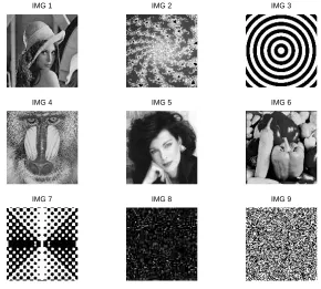
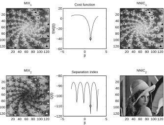
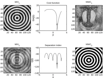
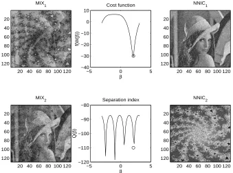
4. Application to Non-Negative Independent Component Analysis: Algorithms Implementation and Numerical Experiments
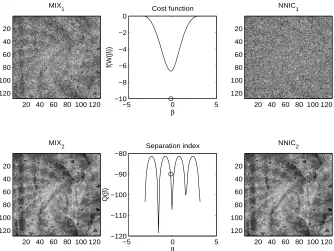
The aims of the present section are to recall the concept of non-negative independent component analysis (ICA+) and the basic related results, to customize the general learning algorithms on the orthogonal group to the case of ICA+, and to present and discuss some numerical cases related to non-negative ICA applied to the separation of gray-level images.
4.1 Non-Negative Independent Component Analysis
Independent component analysis (ICA) is a signal/data processing technique that allows to re-cover independent random processes from their unknown combinations (Cichocki and Amari, 2002; Hyv¨arinen et al., 2001). In particular, standard ICA allows the decomposition of a random process
x(t)∈IRpinto the affine instantaneous model:
x(t) =As(t) +n(t), (18)
where A∈IRp×pis the mixing operator, s(t)∈IRpis the source stream and n(t)∈IRp denotes the disturbance affecting the measurement of x(t)or some nuisance parameters that are not taken into account by the linear part of the model.
The classical hypotheses on the involved quantities are that the mixing operator is full-rank, that at most one among the source signals exhibit Gaussian statistics, and that the source signals are statistically independent at any time. The latter condition may be formally stated through the complete factorization principle, which ensures that the joint probability density function of statisti-cally independent random variables factorizes into the product of their marginal probability density functions. We also add the technical hypothesis that the sources do not have degenerate (that is, point-mass-like) joint probability density function. This implies that for example, the probability that the sources are simultaneously exactly zero is null. Under these hypotheses, it is possible to re-cover the sources up to (usually unessential) re-ordering and scaling, as well as the mixing operator. Neural ICA consists in training an artificial neural network described by y(t) =W(t)x(t), with
Due to the difficulty of measuring the statistical independence of the network’s output signals, several different techniques have been developed in order to perform ICA. The most common ap-proaches to ICA are those based on working out the fourth-order statistics of the network outputs and to the minimization of the (approximate) mutual information among the network’s outputs. The existing approaches invoke some approximations or assumptions in some stage of ICA-algorithm development, most of which concern the (unavailable) structure of the source’s probability distribu-tion.
As it is well-known, a linear, full-rank, noiseless and instantaneous model may be always re-placed by an orthogonal model, in which the mixing matrix A is supposed to belong to O(p). This result may be obtained by pre-whitening the observed signal x, which essentially consists in remov-ing second-order statistical information from the observed signals. When the mixture is orthogonal, the separating network’s connection matrix must also be orthogonal, so we may restrict the learning process to searching the proper connection matrix within O(p).
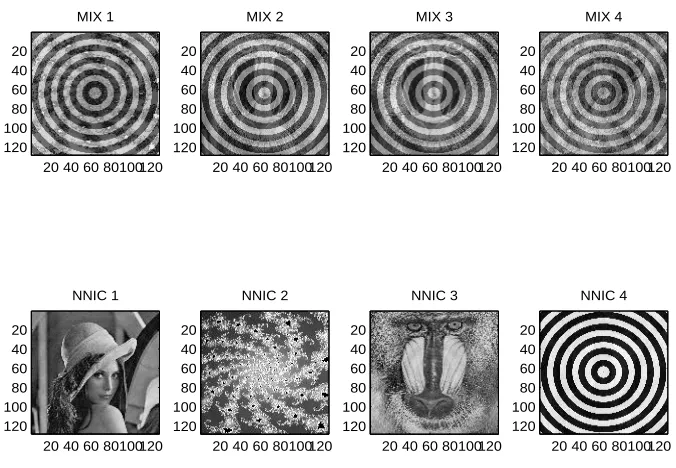
An interesting variant of standard ICA may be invoked when the additional knowledge on the non-negativity of the source signals is considered. In some signal processing situations, in fact, it is a priori known that the sources to be recovered have non-negative values (Plumbley, 2002, 2003). This is the case, for instance, in image processing, where the values of the luminance or the intensity of the color in the proper channel are normally expressed through non-negative integer val-ues. Another interesting potential application is spectral unmixing in remote sensing (Keshava and Mustard, 2002). The evolution of passive remote sensing has witnessed the collection of measure-ments with great spectral resolution, with the aim of extracting increasingly detailed information from pixels in a scene for both civilian and military applications. Pixels of interest are frequently a combination of diverse components: In hyper-spectral imagery, pixels are a mixture of more than one distinct substance. In fact, this may happen if the spatial resolution of a sensor is so low that diverse materials can occupy a single pixel, as well as when distinct materials are combined into a homogeneous mixture. Spectral demixing is the procedure with which the measured spectrum is de-composed into a set of component spectra and a set of corresponding abundances, that indicate the proportion of each component present in the pixels. The theoretical foundations of the non-negative independent component analysis (ICA+) have been given by Plumbley (2002), and then Plumbley (2003) proposed an optimization algorithm for non-negative ICA based on geodesic learning and applied it to the blind separation of three gray-level images. Further recent news on this topic have been published by Plumbley (2004). In our opinion, non-negative ICA as proposed by Plumbley (2003) is an interesting task and, noticeably, it also gives rise to statistical-approximation-free and parameter-free learning algorithms.
Under the hypotheses motivated by Plumbley (2002), a way to perform non-negative indepen-dent component analysis is to construct a cost function f(W) of the network connection matrix that is identically zero if and only if the entries of network’s output signal y are non-negative with probability 1. The criterion function chosen by Plumbley (2003) is f : O(p)→IR+0 defined by
f(W)def=1
2IEx[kx−W
Tρ(Wx)
k2], (19)
where IEx[·]denotes statistical expectation with respect to the statistics of x,k · k2denotes the
stan-dard L2vector norm and the functionρ(·)denotes the ‘rectifier’:
ρ(u)def=
u , if u≥0,