Learning High-Dimensional Markov Forest Distributions:
Analysis of Error Rates
Vincent Y. F. Tan [email protected]
Department of Electrical and Computer Engineering University of Wisconsin-Madison
Madison, WI 53706
Animashree Anandkumar [email protected]
Center for Pervasive Communications and Computing Electrical Engineering and Computer Science University of California, Irvine
Irvine, CA 92697
Alan S. Willsky [email protected]
Stochastic Systems Group
Laboratory for Information and Decision Systems Massachusetts Institute of Technology
Cambridge, MA 02139
Editor: Marina Meil˘a
Abstract
The problem of learning forest-structured discrete graphical models from i.i.d. samples is con-sidered. An algorithm based on pruning of the Chow-Liu tree through adaptive thresholding is proposed. It is shown that this algorithm is both structurally consistent and risk consistent and the error probability of structure learning decays faster than any polynomial in the number of samples under fixed model size. For the high-dimensional scenario where the size of the model d and the number of edges k scale with the number of samples n, sufficient conditions on(n,d,k)are given for the algorithm to satisfy structural and risk consistencies. In addition, the extremal structures for learning are identified; we prove that the independent (resp., tree) model is the hardest (resp., easiest) to learn using the proposed algorithm in terms of error rates for structure learning.
Keywords: graphical models, forest distributions, structural consistency, risk consistency, method
of types
1. Introduction
The challenge in learning graphical models is often compounded by the fact that typically only a small number of samples are available relative to the size of the model (dimension of data). This is referred to as the high-dimensional learning regime, which differs from classical statistics where a large number of samples of fixed dimensionality are available. As a concrete example, in order to analyze the effect of environmental and genetic factors on childhood asthma, clinician scientists in Manchester, UK have been conducting a longitudinal birth-cohort study since 1997 (Custovic et al., 2002; Simpson et al., 2010). The number of variables collected is of the order of d≈106 (dominated by the genetic data) but the number of children in the study is small (n≈103). The paucity of subjects in the study is due in part to the prohibitive cost of collecting high-quality clinical data from willing participants.
In order to learn high-dimensional graphical models, it is imperative to strike the right balance between data fidelity and overfitting. To ameliorate the effect of overfitting, the samples are often fitted to a sparse graphical model (Wainwright and Jordan, 2003), with a small number of edges. One popular and tractable class of sparse graphical models is the set of tree1 models. When re-stricted to trees, the Chow-Liu algorithm (Chow and Liu, 1968; Chow and Wagner, 1973) provides an efficient implementation of the maximum-likelihood (ML) procedure to learn the structure from independent samples. However, in the high-dimensional regime, even a tree may overfit the data (Liu et al., 2011). In this paper, we consider learning high-dimensional, forest-structured (discrete) graphical models from a given set of samples.
For learning the forest structure, the ML (Chow-Liu) algorithm does not produce a consistent estimate since ML favors richer model classes and hence, outputs a tree in general. We propose a consistent algorithm calledCLThres, which has a thresholding mechanism to prune “weak” edges from the Chow-Liu tree. We provide tight bounds on the overestimation and underestimation errors, that is, the error probability that the output of the algorithm has more or fewer edges than the true model.
1.1 Main Contributions
This paper contains three main contributions. Firstly, we propose an algorithm namedCLThresand prove that it is structurally consistent when the true distribution is forest-structured. Secondly, we prove thatCLThresis risk consistent, meaning that the risk under the estimated model converges to the risk of the forest projection2 of the underlying distribution, which may not be a forest. We also provide precise convergence rates for structural and risk consistencies. Thirdly, we provide conditions for the consistency ofCLThresin the high-dimensional setting.
We first prove thatCLThresis structurally consistent, i.e., as the number of samples grows for a fixed model size, the probability of learning the incorrect structure (set of edges), decays to zero for a fixed model size. We show that the error rate is in fact, dominated by the rate of decay of the overestimation error probability.3 We use an information-theoretic technique known as the method
of types (Cover and Thomas, 2006, Ch. 11) as well as a recently-developed technique known as
Euclidean information theory (Borade and Zheng, 2008). We provide an upper bound on the error probability by using convex duality to find a surprising connection between the overestimation error
1. A tree is a connected, acyclic graph. We use the term proper forest to denote the set of disconnected, acyclic graphs. 2. The forest projection is the forest-structured graphical model that is closest in the KL-divergence sense to the true
distribution. We define this distribution formally in (12).
rate and a semidefinite program (Vandenberghe and Boyd, 1996) and show that the overestimation error in structure learning decays faster than any polynomial in n for a fixed data dimension d.
We then consider the high-dimensional scenario and provide sufficient conditions on the growth of(n,d) (and also the true number of edges k) to ensure that CLThres is structurally consistent. We prove that even if d grows faster than any polynomial in n (and in fact close to exponential in
n), structure estimation remains consistent. As a corollary from our analyses, we also show that
forCLThres, independent models (resp., tree models) are the “hardest” (resp., “easiest”) to learn in the sense that the asymptotic error rate is the highest (resp., lowest), over all models with the same scaling of(n,d). Thus, the empty graph and connected trees are the extremal forest structures for learning. We also prove thatCLThresis risk consistent, i.e., the risk of the estimated forest distribu-tion converges to the risk of the forest projecdistribu-tion of the true model at a rate of Op(d log d/n1−γ)for
anyγ>0. We compare and contrast this rate to existing results such as Liu et al. (2011). Note that for this result, the true probability model does not need to be a forest-structured distribution. Finally, we useCLThresto learn forest-structured distributions given synthetic and real-world data sets and show that in the finite-sample case, there exists an inevitable trade-off between the underestimation and overestimation errors.
1.2 Related Work
There are many papers that discuss the learning of graphical models from data. See Dudik et al. (2004), Lee et al. (2006), Abbeel et al. (2006), Wainwright et al. (2006), Meinshausen and Buehlmann (2006), Johnson et al. (2007), and references therein. Most of these methods pose the learning prob-lem as a parameterized convex optimization probprob-lem, typically with a regularization term to enforce sparsity in the learned graph. Consistency guarantees in terms of n and d (and possibly the max-imum degree) are provided. Information-theoretic limits for learning graphical models have also been derived in Santhanam and Wainwright (2008). In Zuk et al. (2006), bounds on the error rate for learning the structure of Bayesian networks using the Bayesian Information Criterion (BIC) were provided. Bach and Jordan (2003) learned tree-structured models for solving the indepen-dent component analysis (ICA) problem. A PAC analysis for learning thin junction trees was given in Chechetka and Guestrin (2007). Meil˘a and Jordan (2000) discussed the learning of graphical models from a different perspective; namely that of learning mixtures of trees via an expectation-maximization procedure.
By using the theory of large-deviations (Dembo and Zeitouni, 1998; Den Hollander, 2000), we derived and analyzed the error exponent for learning trees for discrete (Tan et al., 2011) and Gaussian (Tan et al., 2010a) graphical models. The error exponent is a quantitative measure of performance of the learning algorithm since a larger exponent implies a faster decay of the error probability. However, the analysis does not readily extend to learning forest models and furthermore it was for the scenario when number of variables d does not grow with the number of samples n. In addition, we also posed the structure learning problem for trees as a composite hypothesis testing problem (Tan et al., 2010b) and derived a closed-form expression for the Chernoff-Stein exponent in terms of the mutual information on the bottleneck edge.
error rates for structure learning via the method of types, a powerful proof technique in information theory and statistics. We compare our convergence rates to these related works in Section 6. Further-more, the algorithm suggested in both papers uses a subset (usually half) of the data set to learn the full tree model and then uses the remaining subset to prune the model based on the log-likelihood on the held-out set. We suggest a more direct and consistent method based on thresholding, which uses the entire data set to learn and prune the model without recourse to validation on a held-out data set. It is well known that validation is both computationally expensive (Bishop, 2008, pp. 33) and a potential waste of valuable data which may otherwise be employed to learn a better model. In Liu et al. (2011), the problem of estimating forests with restricted component sizes was considered and was proven to be NP-hard. We do not restrict the component size in this paper but instead attempt to learn the model with the minimum number of edges which best fits the data.
Our work is also related to and inspired by the vast body of literature in information theory and statistics on Markov order estimation. In these works, the authors use various regularization and model selection schemes to find the optimal order of a Markov chain (Merhav et al., 1989; Finesso et al., 1996; Csisz´ar and Shields, 2000), hidden Markov model (Gassiat and Boucheron, 2003) or exponential family (Merhav, 1989). We build on some of these ideas and proof techniques to identify the correct set of edges (and in particular the number of edges) in the forest model and also to provide strong theoretical guarantees of the rate of convergence of the estimated forest-structured distribution to the true one.
1.3 Organization of Paper
This paper is organized as follows: We define the mathematical notation and formally state the prob-lem in Section 2. In Section 3, we describe the algorithm in full detail, highlighting its most salient aspect—the thresholding step. We state our main results on error rates for structure learning in Sec-tion 4 for a fixed forest-structured distribuSec-tion. We extend these results to the high-dimensional case when(n,d,k)scale in Section 5. Extensions to rates of convergence of the estimated distribution, that is, the order of risk consistency, are discussed briefly in Section 6. Numerical simulations on synthetic and real data are presented in Section 7. Finally, we conclude the discussion in Section 8. The proofs of the majority of the results are provided in the appendices.
2. Preliminaries and Problem Formulation
Let G= (V,E)be an undirected graph with vertex (or node) set V :={1, . . . ,d}and edge set E⊂ V2 and let nbd(i):={j∈V :(i,j)∈E}be the set of neighbors of vertex i. Let the set of labeled trees (connected, acyclic graphs) with d nodes beTd and let the set of forests (acyclic graphs) with k
edges and d nodes be Td
k for 0≤k≤d−1. The set of forests includes all the trees. We reserve
the term proper forests for the set of disconnected acylic graphs∪d−2
k=0Tkd. We also use the notation Fd:=∪d−1
k=0Tkdto denote the set of labeled forests with d nodes.
A graphical model (Lauritzen, 1996) is a family of multivariate probability distributions (prob-ability mass functions) in which each distribution factorizes according to a given undirected graph and where each variable is associated to a node in the graph. LetX={1, . . . ,r}(where 2≤r<∞) be a finite set andXd the d-fold Cartesian product of the set X. As usual, let P(Xd) denote the
distribution Q∈P(Xd)is Markov on the graph G= (V,E)if
Q(xi|xnbd(i)) =Q(xi|xV\i), ∀i∈V, (1)
where xV\i is the collection of variables excluding variable i. Equation (1) is known as the local Markov property (Lauritzen, 1996). In this paper, we always assume that graphs are minimal rep-resentations for the corresponding graphical model, that is, if Q is Markov on G, then G has the
smallest number of edges for the conditional independence relations in (1) to hold. We say the distribution Q is a forest-structured distribution if it is Markov on a forest. We also use the nota-tion D(Tkd)⊂P(Xd)to denote the set of d-variate distributions Markov on a forest with k edges. Similarly,D(Fd)is the set of forest-structured distributions.
Let P∈D(Td
k) be a discrete forest-structured distribution Markov on TP = (V,EP)∈Tdk (for
some k=0, . . . ,d−1). It is known that the joint distribution P factorizes as follows (Lauritzen, 1996; Wainwright and Jordan, 2003):
P(x) =
∏
i∈V
Pi(xi)
∏
(i,j)∈EP
Pi,j(xi,xj) Pi(xi)Pj(xj)
,
where{Pi}i∈V and{Pi,j}(i,j)∈EP are the node and pairwise marginals which are assumed to be
posi-tive everywhere.
The mutual information (MI) of two random variables Xi and Xj with joint distribution Pi,j is
the function I(·):P(X2)→[0,log r]defined as
I(Pi,j):=
∑
(xi,xj)∈X2
Pi,j(xi,xj)log
Pi,j(xi,xj) Pi(xi)Pj(xj)
. (2)
This notation for mutual information differs from the usual I(Xi; Xj) used in Cover and Thomas
(2006); we emphasize the dependence of I on the joint distribution Pi,j. The minimum mutual information in the forest, denoted as Imin:=min(i,j)∈EPI(Pi,j) will turn out to be a fundamental
quantity in the subsequent analysis. Note from our minimality assumption that Imin>0 since all edges in the forest have positive mutual information (none of the edges are degenerate). When we consider the scenario where d grows with n in Section 5, we assume that Iminis uniformly bounded away from zero.
2.1 Problem Statement
We now state the basic problem formally. We are given a set of i.i.d. samples, denoted as xn:= {x1, . . . ,xn}. Each sample xl= (xl,1, . . . ,xl,d)∈Xdis drawn independently from P∈D(Tkd)a
forest-structured distribution. From these samples, and the prior knowledge that the undirected graph is acyclic (but not necessarily connected), estimate the true set of edges EP as well as the true
distribution P consistently.
3. The Forest Learning Algorithm: CLThres
We now describe our algorithm for estimating the edge set EPand the distribution P. This algorithm
tree-structured distributions (Chow and Liu, 1968). We call our algorithmCLThreswhich stands for Chow-Liu with Thresholding.
The inputs to the algorithm are the set of samples xnand a regularization sequence{εn}n∈N(to
be specified precisely later) that typically decays to zero, that is, limn→∞εn=0. The outputs are the
estimated edge set, denotedEbbk
n, and the estimated distribution, denoted P
∗.
1. Given xn, calculate the set of pairwise empirical distributions4(or pairwise types){Pbi,j}i,j∈V.
This is just a normalized version of the counts of each observed symbol inX2and serves as a set of sufficient statistics for the estimation problem. The dependence ofPbi,j on the samples xnis suppressed.
2. Form the set of empirical mutual information quantities:
I(Pbi,j):=
∑
(xi,xj)∈X2 b
Pi,j(xi,xj)log b
Pi,j(xi,xj) b
Pi(xi)Pbj(xj)
,
for 1≤i,j≤d. This is a consistent estimator of the true mutual information in (2).
3. Run a max-weight spanning tree (MWST) algorithm (Prim, 1957; Kruskal, 1956) to obtain an estimate of the edge set:
b
Ed−1:= argmax
E:T=(V,E)∈Td (i,
∑
j)∈EI(Pbi,j).
Let the estimated edge set beEbd−1:={be1, . . . ,bed−1}where the edges bei are sorted
accord-ing to decreasaccord-ing empirical mutual information values. We index the edge set by d−1 to emphasize that it has d−1 edges and hence is connected. We denote the sorted empirical mutual information quantities as I(Pbbe1)≥. . .≥I(Pbbed−1). These first three steps constitute the
Chow-Liu algorithm (Chow and Liu, 1968).
4. Estimate the true number of edges using the thresholding estimator:
b
kn:= argmin
1≤j≤d−1
n
I(Pbebj): I(Pbebj)≥εn,I(Pbbej+1)≤εn
o
. (3)
If there exists an empirical mutual information I(Pbbej) such that I(Pbbej) =εn, break the tie
arbitrarily.5
5. Prune the tree by retaining only the topbknedges, that is, define the estimated edge set of the
forest to be
b Ebk
n :={be1, . . . ,bebkn},
where{bei: 1≤i≤d−1} is the ordered edge set defined in Step 3. Define the estimated
forest to beTbbk
n:= (V,Ebbkn).
4. In this paper, the terms empirical distribution and type are used interchangeably.
6. Finally, define the estimated distribution P∗to be the reverse I-projection (Csisz´ar and Mat´uˇs, 2003) of the joint typeP ontob Tbbk
n, that is,
P∗(x):= argmin
Q∈D(Tbbkn)
D(Pb||Q).
It can easily be shown that the projection can be expressed in terms of the marginal and pairwise joint types:
P∗(x) =
∏
i∈V b
Pi(xi)
∏
(i,j)∈Ebbkn b
Pi,j(xi,xj) b
Pi(xi)Pbj(xj)
.
Intuitively,CLThresfirst constructs a connected tree(V,Ebd−1)via Chow-Liu (in Steps 1–3) before pruning the weak edges (with small mutual information) to obtain the final structure Ebbk
n. The
estimated distribution P∗is simply the ML estimate of the parameters subject to the constraint that
P∗is Markov on the learned treeTbbk
n.
Note that if Step 4 is omitted andbkn is defined to be d−1, thenCLThressimply reduces to the
Chow-Liu ML algorithm. Of course Chow-Liu, which outputs a tree, is guaranteed to fail (not be structurally consistent) if the number of edges in the true model k<d−1, which is the problem of interest in this paper. Thus, Step 4, a model selection step, is essential in estimating the true number of edges k. This step is a generalization of the test for independence of discrete memoryless sources discussed in Merhav (1989). In our work, we exploit the fact that the empirical mutual information
I(Pbbej)corresponding to a pair of independent variablesbejwill be very small when n is large, thus a
thresholding procedure using the (appropriately chosen) regularization sequence{εn}will remove
these edges. In fact, the subsequent analysis allows us to conclude that Step 4, in a formal sense,
dominates the error probability in structure learning. CLThres is also efficient as shown by the following result.
Proposition 1 (Complexity ofCLThres) CLThresruns in time O((n+log d)d2).
Proof The computation of the sufficient statistics in Steps 1 and 2 requires O(nd2)operations. The MWST algorithm in Step 3 requires at most O(d2log d) operations (Prim, 1957). Steps 4 and 5 simply require the sorting of the empirical mutual information quantities on the learned tree which only requires O(log d)computations.
4. Structural Consistency For Fixed Model Size
In this section, we keep d and k fixed and consider a probability model P, which is assumed to be Markov on a forest inTdk. This is to gain better insight into the problem before we analyze the high-dimensional scenario in Section 5 where d and k scale6with the sample size n. More precisely, we are interested in quantifying the rate at which the probability of the error event of structure learning
An:=nxn∈(Xd)n:Ebbk
n(x n)6=E
P o
(4)
decays to zero as n tends to infinity. Recall that Ebbk
n, with cardinalitybkn, is the learned edge set
by using CLThres. As usual, Pn is the n-fold product probability measure corresponding to the forest-structured distribution P.
Before stating the main result of this section in Theorem 3, we first state an auxiliary result that essentially says that if one is provided with oracle knowledge of Imin, the minimum mutual information in the forest, then the problem is greatly simplified.
Proposition 2 (Error Rate with knowledge of Imin) Assume that Iminis known inCLThres. Then
by letting the regularization sequence beεn=Imin/2 for all n, we have lim
n→∞ 1
nlog P n(A
n)<0, (5)
that is, the error probability decays exponentially fast.
The proof of this theorem and all other results in the sequel can be found in the appendices. Thus, the primary difficulty lies in estimating Iminor equivalently, the number of edges k. Note that if k is known, a simple modification to the Chow-Liu procedure by imposing the constraint that the final structure contains k edges will also yield exponential decay as in (5). However, in the realistic case where both Iminand k are unknown, we show in the rest of this section that we can design the regularization sequenceεnin such a way that the rate of decay of Pn(An)decays almost
exponentially fast.
4.1 Error Rate for Forest Structure Learning
We now state one of the main results in this paper. We emphasize that the following result is stated for a fixed forest-structured distribution P∈D(Td
k)so d and k are also fixed natural numbers.
Theorem 3 (Error Rate for Structure Learning) Assume that the regularization sequence{εn}n∈N
satisfies the following two conditions:
lim
n→∞εn=0, nlim→∞
nεn
log n=∞. (6)
Then, if the true model TP= (V,EP)is a proper forest (k<d−1), there exists a constant CP∈(1,∞) such that
−CP≤lim inf n→∞
1
nεn
log Pn(An) (7)
≤lim sup
n→∞ 1
nεn
log Pn(An)≤ −1. (8)
Finally, if the true model TP= (V,EP)is a tree (k=d−1), then
lim
n→∞ 1
nlog P n(A
n)<0, (9)
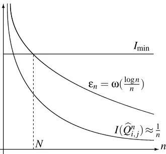
-6
n Imin
εn=ω(log nn )
I(Qbni,j)≈1n
N
Figure 1: Graphical interpretation of the condition onεn. As n→∞, the regularization sequenceεn
will be smaller than Iminand larger than I(Qbni,j)with high probability.
4.2 Interpretation of Result
From (8), the rate of decay of the error probability for proper forests is subexponential but nonethe-less can be made faster than any polynomial for an appropriate choice ofεn. The reason for the
subexponential rate is because of our lack of knowledge of Imin, the minimum mutual information in the true forest TP. For trees, the rate7is exponential (=. exp(−nF)for some positive constant F).
Learning proper forests is thus, strictly “harder” than learning trees. The condition onεnin (6) is
needed for the following intuitive reasons:
1. Firstly, (6) ensures that for all sufficiently large n, we haveεn <Imin. Thus, the true edges will be correctly identified byCLThresimplying that with high probability, there will not be underestimation as n→∞.
2. Secondly, for two independent random variables Xi and Xj with distribution Qi,j =QiQj,
the sequence8 σ(I(Qbni,j)) =Θ(1/n), where Qbni,j is the joint empirical distribution of n i.i.d. samples drawn from Qi,j. Since the regularization sequence εn=ω(log n/n) has a slower
rate of decay thanσ(I(Qbni,j)),εn>I(Qbni,j) with high probability as n→∞. Thus, with high
probability there will not be overestimation as n→∞.
See Figure 1 for an illustration of this intuition. The formal proof follows from a method of types argument and we provide an outline in Section 4.3. A convenient choice ofεnthat satisfies (6) is
εn:=n−β, ∀β∈(0,1). (10)
Note further that the upper bound in (8) is also independent of P since it is equal to −1 for all P. Thus, (8) is a universal result for all forest distributions P∈D(Fd). The intuition for this
7. We use the asymptotic notation from information theory=. to denote equality to first order in the exponent. More precisely, for two positive sequences{an}n∈Nand{bn}n∈Nwe say that an=. bniff limn→∞n−1log(an/bn) =0.
8. The notationσ(Z)denotes the standard deviation of the random variable Z. The fact that the standard deviation of the empirical MIσ(I(Qbni,j))decays as 1/n can be verified by Taylor expanding I(Qbni,j)around Qi,j=QiQjand using
universality is because in the large-n regime, the typical way an error occurs is due to overestimation. The overestimation error results from testing whether pairs of random variables are independent and our asymptotic bound for the error probability of this test does not depend on the true distribution
P.
The lower bound CP in (7), defined in the proof in Appendix B, means that we cannot hope to
do much better usingCLThresif the original structure (edge set) is a proper forest. Together, (7) and (8) imply that the rate of decay of the error probability for structure learning is tight to within a constant factor in the exponent. We believe that the error rates given in Theorem 3 cannot, in general, be improved without knowledge of Imin. We state a converse (a necessary lower bound on sample complexity) in Theorem 7 by treating the unknown forest graph as a uniform random variable over all possible forests of fixed size.
4.3 Proof Idea
The method of proof for Theorem 3 involves using the Gallager-Fano bounding technique (Fano, 1961, pp. 24) and the union bound to decompose the overall error probability Pn(An) into three distinct terms: (i) the rate of decay of the error probability for learning the top k edges (in terms of the mutual information quantities) correctly—known as the Chow-Liu error, (ii) the rate of decay of the overestimation error{bkn>k}and (iii) the rate of decay of the underestimation error{bkn<k}.
Each of these terms is upper bounded using a method of types (Cover and Thomas, 2006, Ch. 11) argument. It turns out, as is the case with the literature on Markov order estimation (e.g., Finesso et al., 1996), that bounding the overestimation error poses the greatest challenge. Indeed, we show that the underestimation and Chow-Liu errors have exponential decay in n. However, the overestimation error has subexponential decay (≈exp(−nεn)).
The main technique used to analyze the overestimation error relies on Euclidean information
theory (Borade and Zheng, 2008) which states that if two distributionsν0andν1(both supported on a common finite alphabetY) are close entry-wise, then various information-theoretic measures can be approximated locally by quantities related to Euclidean norms. For example, the KL-divergence
D(ν0||ν1)can be approximated by the square of a weighted Euclidean norm:
D(ν0||ν1) = 1 2a
∑
∈Y(ν0(a)−ν1(a))2
ν0(a) +o(kν0−ν1k 2
∞). (11)
Note that ifν0≈ν1, then D(ν0||ν1)is close to the sum in (11) and the o(kν0−ν1k2∞)term can be neglected. Using this approximation and Lagrangian duality (Bertsekas, 1999), we reduce a non-convex I-projection (Csisz´ar and Mat´uˇs, 2003) problem involving information-theoretic quantities (such as divergence) to a relatively simple semidefinite program (Vandenberghe and Boyd, 1996) which admits a closed-form solution. Furthermore, the approximation in (11) becomes exact as
n→∞(i.e.,εn→0), which is the asymptotic regime of interest. The full details of the proof can be
found Appendix B.
4.4 Error Rate for Learning the Forest Projection
forests (or forest projection) to be
e
P :=argmin
Q∈D(Fd)
D(P||Q). (12)
If there are multiple optimizing distribution, choose a projectionP that is minimal, that is, its graphe TPe= (V,EPe)has the fewest number of edges such that (12) holds. If we redefine the eventAnin (4)
to beAen:={Ebbk
n6=EPe}, we have the following analogue of Theorem 3.
Corollary 4 (Error Rate for Learning Forest Projection) Let P be an arbitrary distribution and
the eventAenbe defined as above. Then the conclusions in (7)–(9) in Theorem 3 hold if the regular-ization sequence{εn}n∈Nsatisfies (6).
5. High-Dimensional Structural Consistency
In the previous section, we considered learning a fixed forest-structured distribution P (and hence fixed d and k) and derived bounds on the error rate for structure learning. However, for most problems of practical interest, the number of data samples is small compared to the data dimension
d (see the asthma example in the introduction). In this section, we prove sufficient conditions on
the scaling of(n,d,k) for structure learning to remain consistent. We will see that even if d and
k are much larger than n, under some reasonable regularity conditions, structure learning remains
consistent.
5.1 Structure Scaling Law
To pose the learning problem formally, we consider a sequence of structure learning problems in-dexed by the number of data points n. For the particular problem inin-dexed by n, we have a data set
xn= (x1, . . . ,xn) of size n where each sample xl ∈Xd is drawn independently from an unknown d-variate forest-structured distribution P(d)∈D(Tkd), which has d nodes and k edges and where d and k depend on n. This high-dimensional setup allows us to model and subsequently analyze how
d and k can scale with n while maintaining consistency. We will sometimes make the dependence
of d and k on n explicit, that is, d=dnand k=kn.
In order to be able to learn the structure of the models we assume that
(A1) Iinf:= inf
d∈N(i,jmin)∈E P(d)
I(Pi(,dj))>0, (13)
(A2) κ:= inf
d∈Nximin,xj∈XP (d)
i,j (xi,xj)>0. (14)
That is, assumptions (A1) and (A2) insure that there exists uniform lower bounds on the minimum mutual information and the minimum entry in the pairwise probabilities in the forest models as the size of the graph grows. These are typical regularity assumptions for the high-dimensional setting. See Wainwright et al. (2006) and Meinshausen and Buehlmann (2006) for example. We again emphasize that the proposed learning algorithm CLThreshas knowledge of neither Iinf nor
κ. Equipped with (A1) and (A2) and assuming the asymptotic behavior ofεnin (6), we claim the
Theorem 5 (Structure Scaling Law) There exists two finite, positive constants C1,C2such that if
n>max
n
(2 log(d−k))1+ζ,C1log d,C2log k
o
, (15)
for anyζ>0, then the error probability of incorrectly learning the sequence of edge sets{EP(d)}d∈N
tends to zero as (n,d,k)→∞. When the sequence of forests are trees, n>C log d (where C := max{C1,C2}) suffices for high-dimensional structure recovery.
Thus, if the model parameters(n,d,k)all grow with n but d=o(exp(n/C1)), k=o(exp(n/C2)) and d−k=o(exp(n1−β/2))(for allβ>0), consistent structure recovery is possible in high dimen-sions. In other words, the number of nodes d can grow faster than any polynomial in the sample size n. In Liu et al. (2011), the bivariate densities are modeled by functions from a H¨older class with exponent α and it was mentioned (in Theorem 4.3) that the number of variables can grow like o(exp(nα/(1+α)))for structural consistency. Our result is somewhat stronger but we model the pairwise joint distributions as (simpler) probability mass functions (the alphabetXis a finite set).
5.2 Extremal Forest Structures
In this subsection, we study the extremal structures for learning, that is, the structures that, roughly speaking, lead to the largest and smallest error probabilities for structure learning. Define the se-quence
hn(P):=
1
nεn
log Pn(An), ∀n∈N. (16)
Note that hnis a function of both the number of variables d=dnand the number of edges k=knin
the models P(d)since it is a sequence indexed by n. In the next result, we assume(n,d,k)satisfies the scaling law in (15) and answer the following question: How does hnin (16) depend on the number
of edges knfor a given dn? Let P1(d)and P2(d)be two sequences of forest-structured distributions with
a common number of nodes dnand number of edges kn(P1(d))and kn(P2(d))respectively.
Corollary 6 (Extremal Forests) Assume that CLThres is employed as the forest learning
algo-rithm. As n→∞, hn(P1(d))≤hn(P2(d))whenever kn(P1(d))≥kn(P2(d))implying that hn is maximized when P(d)are product distributions (i.e., kn=0) and minimized when P(d)are tree-structured dis-tributions (i.e., kn=dn−1). Furthermore, if kn(P1(d)) =kn(P2(d)), then hn(P1(d)) =hn(P2(d)).
Note that the corollary is intimately tied to the proposed algorithmCLThres.We are not claiming that such a result holds for all other forest learning algorithms. The intuition for this result is the following: We recall from the discussion after Theorem 3 that the overestimation error dominates the probability of error for structure learning. Thus, the performance of CLThresdegrades with the number of missing edges. If there are very few edges (i.e., knis very small relative to dn), the
CLThresestimator is more likely to overestimate the number of edges as compared to if there are many edges (i.e., kn/dnis close to 1). We conclude that a distribution which is Markov on an empty graph (all variables are independent) is the hardest to learn (in the sense of Corollary 6 above).
Conversely, trees are the easiest structures to learn.
5.3 Lower Bounds on Sample Complexity
possible over all algorithms (estimators). To answer this question, we limit ourselves to the scenario where the true graph TP is a uniformly distributed chance variable9 with probability measure P.
Assume two different scenarios:
(a) TP is drawn from the uniform distribution onTkd, that is, P(TP=t) =1/|Tdk|for all forests t∈Tkd. Recall thatTkdis the set of labeled forests with d nodes and k edges.
(b) TP is drawn from the uniform distribution on Fd, that is, P(TP=t) =1/|Fd|for all forests t∈Fd. Recall thatFdis the set of labeled forests with d nodes.
This following result is inspired by Theorem 1 in Bresler et al. (2008). Note that an estimator or
algorithmTbd is simply a map from the set of samples(Xd)n to a set of graphs (eitherTd
k orFd).
We emphasize that the following result is stated with the assumption that we are averaging over the random choice of the true graph TP.
Theorem 7 (Lower Bounds on Sample Complexity) Letρ<1 and r :=|X|. In case (a) above, if
n<ρ(k−1)log d
d log r , (17)
thenP(Tbd6=TP)→1 for any estimatorTbd:(Xd)n→Td
k. Alternatively, in case (b), if
n<ρlog d
log r, (18)
thenP(Tbd6=TP)→1 for any estimatorTbd:(Xd)n→Fd.
This result, a strong converse, states that n=Ω(k
dlog d) is necessary for any estimator with
oracle knowledge of k to succeed. Thus, we need at least logarithmically many samples in d if the fraction k/d is kept constant as the graph size grows even if k is known precisely and does not
have to be estimated. Interestingly, (17) says that if k is large, then we need more samples. This is because there are fewer forests with a small number of edges as compared to forests with a large number of edges. In contrast, the performance ofCLThresdegrades when k is small because it is more sensitive to the overestimation error. Moreover, if the estimator does not know k, then (18) says that n=Ω(log d) is necessary for successful recovery. We conclude that the set of scaling requirements prescribed in Theorem 5 is almost optimal. In fact, if the true structure TP is a tree,
then Theorem 7 for CLThres says that the (achievability) scaling laws in Theorem 5 are indeed optimal (up to constant factors in the O and Ω-notation) since n>(2 log(d−k))1+ζ in (15) is trivially satisfied. Note that if TPis a tree, then the Chow-Liu ML procedure orCLThresresults in
the sample complexity n=O(log d)(see Theorem 5).
6. Risk Consistency
In this section, we develop results for risk consistency to study how fast the parameters of the estimated distribution converge to their true values. For this purpose, we define the risk of the estimated distribution P∗(with respect to the true probability model P) as
Rn(P∗):=D(P||P∗)−D(P||Pe), (19)
9. The term chance variable, attributed to Gallager (2001), describes random quantities Y :Ω→W that take on values
whereP is the forest projection of P defined in (12). Note that the original probability model P doese
not need to be a forest-structured distribution in the definition of the risk. Indeed, if P is Markov on a forest, (19) reduces toRn(P∗) =D(P||P∗)since the second term is zero. We quantify the rate of decay of the risk when the number of samples n tends to infinity. Forδ>0, we define the event
Cn,δ:=
xn∈(Xd)n:Rn(P ∗)
d >δ
. (20)
That is,Cn,δ is the event that the average riskRn(P∗)/d exceeds some constantδ. We say that the estimator P∗(or an algorithm) isδ-risk consistent if the probability ofCn,δtends to zero as n→∞. Intuitively, achieving δ-risk consistency is easier than achieving structural consistency since the learned model P∗ can be close to the true forest-projectionP in the KL-divergence sense even ife
their structures differ.
In order to quantify the rate of decay of the risk in (19), we need to define some stochastic order notation. We say that a sequence of random variables Yn=Op(gn)(for some deterministic positive
sequence{gn}) if for everyε>0, there exists a B=Bε>0 such that lim supn→∞Pr(|Yn|>Bgn)<ε.
Thus, Pr(|Yn|>Bgn)≥εholds for only finitely many n.
We say that a reconstruction algorithm has risk consistency of order (or rate) gn ifRn(P∗) = Op(gn). The definition of the order of risk consistency involves the true model P. Intuitively, we
expect that as n→∞, the estimated distribution P∗converges to the projectionP soe Rn(P∗)→0 in probability.
6.1 Error Exponent for Risk Consistency
In this subsection, we consider a fixed distribution P and state consistency results in terms of the eventCn,δ. Consequently, the model size d and the number of edges k are fixed. This lends in-sight into deriving results for the order of the risk consistency and provides intuition for the high-dimensional scenario in Section 6.2.
Theorem 8 (Error Exponent forδ-Risk Consistency) ForCLThres, there exists a constantδ0> 0 such that for all 0<δ<δ0,
lim sup
n→∞ 1
nlog P n(C
n,δ)≤ −δ. (21)
The corresponding lower bound is
lim inf
n→∞ 1
nlog P n(C
n,δ)≥ −δd. (22)
The theorem states that ifδis sufficiently small, the decay rate of the probability ofCn,δis expo-nential, hence clearlyCLThresisδ-risk consistent. Furthermore, the bounds on the error exponent associated to the eventCn,δ are independent of the parameters of P and only depend onδand the dimensionality d. Intuitively, (21) is true because if we want the risk of P∗to be at most δd, then
each of the empirical pairwise marginals Pbi,j should be δ-close to the true pairwise marginalPei,j.
6.2 The High-Dimensional Setting
We again consider the high-dimensional setting where the tuple of parameters (n,dn,kn) tend to
infinity and we have a sequence of learning problems indexed by the number of data points n. We again assume that (13) and (14) hold and derive sufficient conditions under which the probability of the eventCn,δtends to zero for a sequence of d-variate distributions{P(d)∈P(Xd)}
d∈N. The proof
of Theorem 8 leads immediately to the following corollary.
Corollary 9 (δ-Risk Consistency Scaling Law) Letδ>0 be a sufficiently small constant and a∈ (0,δ). If the number of variables in the sequence of models{P(d)}d∈Nsatisfies dn=o(exp(an)),
thenCLThresisδ-risk consistent for{P(d)}d∈N.
Interestingly, this sufficient condition on how number of variables d should scale with n for consistency is very similar to Theorem 5. In particular, if d is polynomial in n, thenCLThresis both structurally consistent as well asδ-risk consistent. We now study the order of the risk consistency ofCLThresas the model size d grows.
Theorem 10 (Order of Risk Consistency) The risk of the sequence of estimated distributions{(P(d))∗}d∈N
with respect to{P(d)}d∈Nsatisfies
Rn((P(d))∗) =Op
d log d n1−γ
, (23)
for everyγ>0, that is, the risk consistency forCLThresis of order(d log d)/n1−γ.
Note that since this result is stated for the high-dimensional case, d =dn is a sequence in n
but the dependence on n is suppressed for notational simplicity in (23). This result implies that if d=o(n1−2γ)thenCLThresis risk consistent, that is,Rn((P(d))∗)→0 in probability. Note that this result is not the same as the conclusion of Corollary 9 which refers to the probability that the average risk is greater than a fixed constantδ. Also, the order of convergence given in (23) does not depend on the true number of edges k. This is a consequence of the result in (21) where the upper bound on the exponent associated to the eventCn,δis independent of the parameters of P.
The order of the risk, or equivalently the rate of convergence of the estimated distribution to the forest projection, is almost linear in the number of variables d and inversely proportional to n. We provide three intuitive reasons to explain why this is plausible: (i) the dimension of the sufficient statistics in a tree-structured graphical model is of order O(d), (ii) the ML estimator of the natural parameters of an exponential family converge to their true values at the rate of Op(n−1/2)
(Ser-fling, 1980, Sec. 4.2.2), and (iii) locally, the KL-divergence behaves like the square of a weighted Euclidean norm of the natural parameters (Cover and Thomas, 2006, Equation (11.320)).
We now compare Theorem 10 to the corresponding results in Liu et al. (2011). In these recent papers, it was shown that by modeling the bivariate densitiesPbi,j as functions from a H¨older class
with exponentα>0 and using a reconstruction algorithm based on validation on a held-out data set, the risk decays at a rate10 ofOe
p(dn−α/(1+2α)), which is slower than the order of risk consistency
in (23). This is due to the need to compute the bivariate densities via kernel density estimation. Furthermore, we model the pairwise joint distributions as discrete probability mass functions and not continuous probability density functions, hence there is no dependence on H¨older exponents.
@ @
@ @
@
w
w
w w
w
w w
w w
X1 X2
X3
X4
X5
Xk+1 .. .
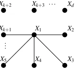
Xk+2 Xk+3 . . . Xd
Figure 2: The forest-structured distribution Markov on d nodes and k edges. Variables Xk+1, . . . ,Xd
are not connected to the main star graph.
7. Numerical Results
In this section, we perform numerical simulations on synthetic and real data sets to study the effect of a finite number of samples on the probability of the eventAndefined in (4). Recall that this is the error event associated to an incorrect learned structure.
7.1 Synthetic Data Sets
In order to compare our estimate to the ground truth graph, we learn the structure of distributions that are Markov on the forest shown in Figure 2. Thus, a subgraph (nodes 1, . . . ,k+1) is a (connected) star while nodes k+2, . . . ,d−1 are not connected to the star. Each random variable Xj takes on
values from a binary alphabetX={0,1}. Furthermore, Pj(xj) =0.5 for xj=0,1 and all j∈V . The
conditional distributions are governed by the “binary symmetric channel”:
Pj|1(xj|x1) =
0.7 xj=x1 0.3 xj6=x1
for j=2, . . . ,k+1. We further assume that the regularization sequence is given byεn:=n−βfor
someβ∈(0,1). Recall that this sequence satisfies the conditions in (6). We will varyβ in our experiments to observe its effect on the overestimation and underestimation errors.
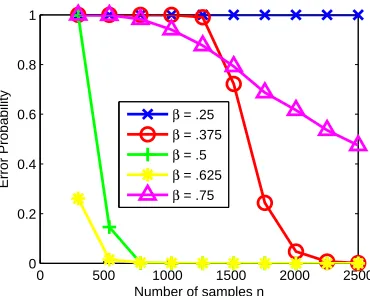
In Figure 3, we show the simulated error probability as a function of the sample size n for a
d=101 node graph (as in Figure 2) with k=50 edges. The error probability is estimated based on 30,000 independent runs ofCLThres(over different data sets xn). We observe that the error
probabil-ity is minimized whenβ≈0.625. Figure 4 show the simulated overestimation and underestimation errors for this experiment. We see that asβ→0, the overestimation (resp., underestimation) error is likely to be small (resp., large) because the regularization sequenceεnis large. When the number of
samples is relatively small as in this experiment, both types of errors contribute significantly to the overall error probability. Whenβ≈0.625, we have the best tradeoff between overestimation and underestimation for this particular experimental setting.
0 500 1000 1500 2000 2500 0
0.2 0.4 0.6 0.8 1
Number of samples n
Error Probability
β = .25 β = .375 β = .5 β = .625 β = .75
Figure 3: The error probability of structure learning forβ∈(0,1).
0 500 1000 1500 2000 2500 0
0.2 0.4 0.6 0.8 1
Number of samples n
Overestimation Error Probability
β = .25 β = .375 β = .5 β = .625 β = .75
0 500 1000 1500 2000 2500 0
0.2 0.4 0.6 0.8 1
Number of samples n
Underestimation Error Probability
β = .25 β = .375 β = .5 β = .625 β = .75
Figure 4: The overestimation and underestimation errors forβ∈(0,1).
samples is very large, it is shown that the overestimation error dominates the overall probability of error and so one should chooseβto be close to zero. The question of how best to select optimalβ when given only a finite number of samples appears to be a challenging one. We use cross-validation as a proxy to select this parameter for the real-world data sets in the next section.
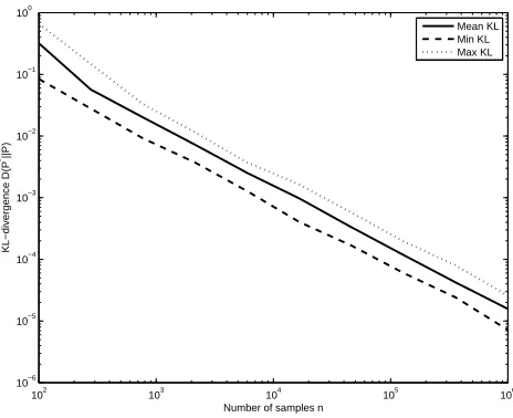
102 103 104 105 106 10−6
10−5 10−4 10−3 10−2
10−1
100
Number of samples n
KL−divergence D(P
*||P)
Mean KL Min KL Max KL
Figure 5: Mean, minimum and maximum (across 50 different runs) of the KL-divergence between the estimated model P∗and the true model P for a d=21 node graph with k=10 edges.
7.2 Real Data Sets
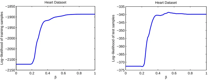
We now demonstrate how well forests-structured distributions can model two real data sets11which are obtained from the UCI Machine Learning Repository (Newman et al., 1998). The first data set we used is known as the SPECT Heart data set, which describes diagnosing of cardiac Single Proton Emission Computed Tomography (SPECT) images on normal and abnormal patients. The data set contains d =22 binary variables and n=80 training samples. There are also 183 test samples. We learned a forest-structured distributions using the 80 training samples for different
β∈(0,1)and subsequently computed the log-likelihood of both the training and test samples. The results are displayed in Figure 6. We observe that, as expected, the log-likelihood of the training samples increases monotonically withβ. This is because there are more edges in the model when
βis large improving the modeling ability. However, we observe that there is overfitting whenβis large as evidenced by the decrease in the log-likelihood of the 183 test samples. The optimal value ofβ in terms of the log-likelihood for this data set is ≈0.25,but surprisingly an approximation with an empty graph12also yields a high log-likelihood score on the test samples. This implies that according to the available data, the variables are nearly independent. The forest graph forβ=0.25 is shown in Figure 7(a) and is very sparse.
The second data set we used is the Statlog Heart data set containing physiological measurements of subjects with and without heart disease. There are 270 subjects and d=13 discrete and contin-uous attributes, such as gender and resting blood pressure. We quantized the contincontin-uous attributes into two bins. Those measurements that are above the mean are encoded as 1 and those below the mean as 0. Since the raw data set is not partitioned into training and test sets, we learned forest-structured models based on a randomly chosen set of n=230 training samples and then computed
11. These data sets are typically employed for binary classification but we use them for modeling purposes.
0 0.2 0.4 0.6 0.8 1 −950
−900 −850 −800 −750 −700 −650
Spect Dataset
β
Log−likelihood of training samples
0 0.2 0.4 0.6 0.8 1 −3500
−3400 −3300 −3200 −3100 −3000 −2900 −2800
Spect Dataset
β
Log−likelihood of test samples
Figure 6: Log-likelihood scores on the SPECT data set
the log-likelihood of these training and 40 remaining test samples. We then chose an additional 49 randomly partitioned training and test sets and performed the same learning task and computa-tion of log-likelihood scores. The mean of the log-likelihood scores over these 50 runs is shown in Figure 8. We observe that the log-likelihood on the test set is maximized atβ≈0.53 and the tree approximation (β≈1) also yields a high likelihood score. The forest learned whenβ=0.53 is shown in Figure 7(b). Observe that two nodes (ECG and Cholesterol) are disconnected from the main graph because their mutual information values with other variables are below the threshold. In contrast, HeartDisease, the label for this data set, has the highest degree, that is, it influences and is influenced by many other covariates. The strengths of the interactions between HeartDisease and its neighbors are also strong as evidenced by the bold edges.
From these experiments, we observe that some data sets can be modeled well as proper forests with very few edges while others are better modeled as distributions that are almost tree-structured (see Figure 7). Also, we need to chooseβcarefully to balance between data fidelity and overfitting. In contrast, our asymptotic result in Theorem 3 says thatεn should be chosen according to (6) so
that we have structural consistency. When the number of data points n is large,β in (10) should be chosen to be small to ensure that the learned edge set is equal to the true one (assuming the underlying model is a forest) with high probability as the overestimation error dominates.
8. Conclusion
F14 F4
F9 F8
F13
F15 F10
F2 F6
F11 F1 F3
F5
F7 F12 F16
F17 F18 F19 F20
F21
F22
Age
RestingBP ColorOfVessels
HeartDisease
Thalassemia ChestPain PeakExercise
Gender Angina Depression MaxHeartRate Cholesterol ECG
(a) (b)
Figure 7: Learned forest graph of the (a) SPECT data set forβ=0.25 and (b) HEART data set for
β=0.53. Bold edges denote higher mutual information values. The features names are not provided for the SPECT data set.
0 0.2 0.4 0.6 0.8 1 −2150
−2100 −2050 −2000 −1950 −1900 −1850
Heart Dataset
β
Log−likelihood of training samples
0 0.2 0.4 0.6 0.8 1 −375
−370 −365 −360 −355 −350 −345 −340 −335
Heart Dataset
β
Log−likelihood of test samples
Acknowledgments
This work was supported by a AFOSR funded through Grant FA9559-08-1-1080, a MURI funded through ARO Grant W911NF-06-1-0076 and a MURI funded through AFOSR Grant FA9550-06-1-0324. V. Tan is also funded by A*STAR, Singapore. The authors would like to thank Sanjoy Mitter, Lav Varshney, Matt Johnson and James Saunderson for discussions. The authors would also like to thank Rui Wu (UIUC) for pointing out an error in the proof of Theorem 3.
Appendix A. Proof of Proposition 2
Proof (Sketch) The proof of this result hinges on the fact that both the overestimation and
under-estimation errors decay to zero exponentially fast when the threshold is chosen to be Imin/2. This threshold is able to differentiate between true edges (with MI larger than Imin) from non-edges (with MI smaller than Imin) with high probability for n sufficiently large. The error for learning the top k edges of the forest also decays exponentially fast (Tan et al., 2011). Thus, (5) holds. The full details of the proof follow in a straightforward manner from Appendix B which we present next.
Appendix B. Proof of Theorem 3
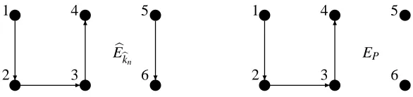
Define the event Bn:={Ebk 6=EP},where Ebk={be1, . . . ,ebk} is the set of top k edges (see Step 3
ofCLThresfor notation). This is the Chow-Liu error as mentioned in Section 4.3. LetBc ndenote
the complement ofBn. Note that inBc
n, the estimated edge set depends on k, the true model order,
which is a-priori unknown to the learner. Further define the constant
KP:= lim n→∞−
1
nlog P n(B
n). (24)
In other words, KP is the error exponent for learning the forest structure incorrectly assuming the
true model order k is known and Chow-Liu terminates after the addition of exactly k edges in the MWST procedure (Kruskal, 1956). The existence of the limit in (24) and the positivity of KPfollow
from the main results in Tan et al. (2011).
We first state a result which relies on the Gallager-Fano bound (Fano, 1961, pp. 24). The proof will be provided at the end of this appendix.
Lemma 11 (Reduction to Model Order Estimation) For everyη∈(0,KP), there exists a N∈N sufficiently large such that for every n>N, the error probability Pn(An)satisfies
(1−η)Pn(bkn6=k|Bcn)≤Pn(An) (25)
≤Pn(bkn6=k|Bcn) +2 exp(−n(KP−η)). (26)
Proof (of Theorem 3) We will prove (i) the upper bound in (8) (ii) the lower bound in (7) and (iii)
the exponential rate of decay in the case of trees (9).
B.1 Proof of Upper Bound in Theorem 3
We now bound the error probability Pn(bkn6=k|Bcn)in (26). Using the union bound,
The first and second terms are known as the overestimation and underestimation errors respectively. We will show that the underestimation error decays exponentially fast. The overestimation error decays only subexponentially fast and so its rate of decay dominates the overall rate of decay of the error probability for structure learning.
B.1.1 UNDERESTIMATIONERROR
We now bound these terms staring with the underestimation error. By the union bound,
Pn(bkn<k|Bcn)≤(k−1) max
1≤j≤k−1P
n(bk
n= j|Bcn)
= (k−1)Pn(bkn=k−1|Bcn), (28)
where (28) follows because Pn(bk
n= j|Bcn)is maximized when j=k−1. This is because if, to the
contrary, Pn(bkn=j|Bcn)were to be maximized at some other j≤k−2, then there exists at least two
edges, call them e1,e2∈EP such that events E1:={I(Pbe1)≤εn}andE2:={I(Pbe2)≤εn}occur.
The probability of this joint event is smaller than the individual probabilities, that is, Pn(E1∩E2)≤ min{Pn(E1),Pn(E2)}. This is a contradiction.
By the rule for choosingbknin (3), we have the upper bound
Pn(bkn=k−1|Bcn) =Pn(∃e∈EP s.t. I(Pbe)≤εn)≤k max e∈EP
Pn(I(Pbe)≤εn), (29)
where the inequality follows from the union bound. Now, note that if e∈EP, then I(Pe)>εn for n sufficiently large (sinceεn→0). Thus, by Sanov’s theorem (Cover and Thomas, 2006, Ch. 11), Pn(I(Pbe)≤εn)can be upper bounded as
Pn(I(Pbe)≤εn)≤(n+1)r
2
exp
−n min
Q∈P(X2){D(Q||Pe): I(Q)≤εn}
. (30)
Define the good rate function (Dembo and Zeitouni, 1998) in (30) to be L :P(X2)×[0,∞)→[0,∞), which is given by
L(Pe; a):= min
Q∈P(X2){D(Q||Pe): I(Q)≤a}. (31)
Clearly, L(Pe; a) is continuous in a. Furthermore it is monotonically decreasing in a for fixed Pe.
Thus by using the continuity of L(Pe;·) we can assert: To everyη>0, there exists a N∈Nsuch
that for all n>N we have L(Pe;εn)>L(Pe; 0)−η. As such, we can further upper bound the error
probability in (30) as
Pn(I(Pbe)≤εn)≤(n+1)r
2
exp(−n(L(Pe; 0)−η)). (32)
By using the fact that Imin>0, the exponent L(Pe; 0)>0 and thus, we can put the pieces in (28),
(29) and (32) together to show that the underestimation error is upper bounded as
Pn(bkn<k|Bnc)≤k(k−1)(n+1)r
2
exp
−n min e∈EP
(L(Pe; 0)−η)
. (33)
Hence, if k is constant, the underestimation error Pn(bkn<k|Bcn) decays to zero exponentially fast
as n→∞, that is, the normalized logarithm of the underestimation error can be bounded as
lim sup
n→∞ 1
nlog P n(bk
n<k|Bcn)≤ −min e∈EP
The above statement is now independent of n. Hence, we can take the limit asη→0 to conclude that:
lim sup
n→∞ 1
nlog P n(bk
n<k|Bcn)≤ −LP. (34)
The exponent LP:=mine∈EPL(Pe; 0)is positive because we assumed that the model is minimal and
so Imin>0, which ensures the positivity of the rate function L(Pe; 0)for each true edge e∈EP.
B.1.2 OVERESTIMATIONERROR
Bounding the overestimation error is harder. It follows by first applying the union bound:
Pn(bkn>k|Bcn)≤(d−k−1) max k+1≤j≤d−1P
n(bk
n= j|Bcn)
= (d−k−1)Pn(bkn=k+1|Bcn), (35)
where (35) follows because Pn(bkn=j|Bcn)is maximized when j=k+1 (by the same argument as
for the underestimation error). Apply the union bound again, we have
Pn(bkn=k+1|Bcn)≤(d−k−1) max e∈V×V :I(Pe)=0
Pn(I(Pbe)≥εn). (36)
From (36), it suffices to bound Pn(I(Pbe)≥εn)for any pair of independent random variables(Xi,Xj)
and e= (i,j). We proceed by applying the upper bound in Sanov’s theorem (Cover and Thomas, 2006, Ch. 11) to Pn(I(Pbe)≥εn)which yields
Pn(I(Pbe)≥εn)≤(n+1)r
2
exp
−n min
Q∈P(X2){D(Q||Pe): I(Q)≥εn}
, (37)
for all n∈N. Our task now is to lower bound the good rate function in (37), which we denote as M :P(X2)×[0,∞)→[0,∞):
M(Pe; b):= min
Q∈P(X2){D(Q||Pe): I(Q)≥b}. (38)
Note that M(Pe; b)is monotonically increasing and continuous in b for fixed Pe. Because the
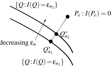
se-quence {εn}n∈N tends to zero, when n is sufficiently large, εn is arbitrarily small and we are in
the so-called very-noisy learning regime (Borade and Zheng, 2008; Tan et al., 2011), where the optimizer to (38), denoted as Q∗n, is very close to Pe. See Figure 9.
Thus, when n is large, the KL-divergence and mutual information can be approximated as
D(Q∗n||Pe) =
1 2v
TΠ
ev+o(kvk2), (39)
I(Q∗n) =1 2v
TH
ev+o(kvk2), (40)
where13v :=vec(Q∗
n)−vec(Pe)∈Rr
2
. The r2×r2matricesΠ
eand Heare defined as
Πe:=diag(1/vec(Pe)), (41) He:=∇2vec(Q)I(vec(Q))
Q=P
e. (42)