Structured Variable Selection with Sparsity-Inducing Norms

Structured Variable Selection with Sparsity-Inducing Norms

Rodolphe Jenatton [email protected]

INRIA - SIERRA Project-team,

Laboratoire d’Informatique de l’Ecole Normale Sup´erieure (INRIA/ENS/CNRS UMR 8548) 23, avenue d’Italie

75214 Paris, France

Jean-Yves Audibert [email protected]

Imagine (ENPC/CSTB), Universit´e Paris-Est,

Laboratoire d’Informatique de l’Ecole Normale Sup´erieure (INRIA/ENS/CNRS UMR 8548) 6 avenue Blaise Pascal

77455 Marne-la-Vall´ee, France

Francis Bach [email protected]

INRIA - SIERRA Project-team,

Laboratoire d’Informatique de l’Ecole Normale Sup´erieure (INRIA/ENS/CNRS UMR 8548), 23, avenue d’Italie

75214 Paris, France

Editor: Bin Yu

Abstract

We consider the empirical risk minimization problem for linear supervised learning, with regular-ization by structured sparsity-inducing norms. These are defined as sums of Euclidean norms on certain subsets of variables, extending the usualℓ1-norm and the groupℓ1-norm by allowing the

subsets to overlap. This leads to a specific set of allowed nonzero patterns for the solutions of such problems. We first explore the relationship between the groups defining the norm and the resul-ting nonzero patterns, providing both forward and backward algorithms to go back and forth from groups to patterns. This allows the design of norms adapted to specific prior knowledge expressed in terms of nonzero patterns. We also present an efficient active set algorithm, and analyze the consistency of variable selection for least-squares linear regression in low and high-dimensional settings.

Keywords: sparsity, consistency, variable selection, convex optimization, active set algorithm

1. Introduction

Sparse linear models have emerged as a powerful framework to deal with various supervised es-timation tasks, in machine learning as well as in statistics and signal processing. These models basically seek to predict an output by linearly combining only a small subset of the features de-scribing the data. To simultaneously address this variable selection and the linear model estimation,

When regularizing by the ℓ1-norm, sparsity is yielded by treating each variable individually,

regardless of its position in the input feature vector, so that existing relationships and structures between the variables (e.g., spatial, hierarchical or related to the physics of the problem at hand) are merely disregarded. However, many practical situations could benefit from this type of prior knowledge, potentially both for interpretability purposes and for improved predictive performance.

For instance, in neuroimaging, one is interested in localizing areas in functional magnetic res-onance imaging (fMRI) or magnetoencephalography (MEG) signals that are discriminative to dis-tinguish between different brain states (Gramfort and Kowalski, 2009; Xiang et al., 2009; Jenatton et al., 2011a, and references therein). More precisely, fMRI responses consist in voxels whose three-dimensional spatial arrangement respects the anatomy of the brain. The discriminative voxels are thus expected to have a specific localized spatial organization (Xiang et al., 2009), which is impor-tant for the subsequent identification task performed by neuroscientists. In this case, regularizing by a plainℓ1-norm to deal with the ill-conditionedness of the problem (typically only a few fMRI responses described by tens of thousands of voxels) would ignore this spatial configuration, with a potential loss in interpretability and performance.

Similarly, in face recognition, robustness to occlusions can be increased by considering as fea-tures, sets of pixels that form small convex regions on the face images (Jenatton et al., 2010b). Again, a plainℓ1-norm regularization fails to encode this specific spatial locality constraint (Jenatton

et al., 2010b). The same rationale supports the use of structured sparsity for background subtraction tasks (Cevher et al., 2008; Huang et al., 2009; Mairal et al., 2010b). Still in computer vision, object and scene recognition generally seek to extract bounding boxes in either images (Harzallah et al., 2009) or videos (Dalal et al., 2006). These boxes concentrate the predictive power associated with the considered object/scene class, and have to be found by respecting the spatial arrangement of the pixels over the images. In videos, where series of frames are studied over time, the temporal coherence also has to be taken into account. An unstructured sparsity-inducing penalty that would disregard this spatial and temporal information is therefore not adapted to select such boxes.

These real world examples motivate the need for the design of sparsity-inducing regulariza-tion schemes, capable of encoding more sophisticated prior knowledge about the expected sparsity patterns.

As mentioned above, the ℓ1-norm focuses only on cardinality and cannot easily specify side

information about the patterns of nonzero coefficients (“nonzero patterns”) induced in the solution, since they are all theoretically possible. Groupℓ1-norms (Yuan and Lin, 2006; Roth and Fischer, 2008; Huang and Zhang, 2010) consider a partition of all variables into a certain number of subsets and penalize the sum of the Euclidean norms of each one, leading to selection of groups rather than individual variables. Moreover, recent works have considered overlapping but nested groups in constrained situations such as trees and directed acyclic graphs (Zhao et al., 2009; Bach, 2008a; Kim and Xing, 2010; Jenatton et al., 2010a, 2011b; Schmidt and Murphy, 2010).

In this paper, we consider all possible sets of groups and characterize exactly what type of prior knowledge can be encoded by considering sums of norms of overlapping groups of variables. Before describing how to go from groups to nonzero patterns (or equivalently zero patterns), we show that it is possible to “reverse-engineer” a given set of nonzero patterns, that is, to build the unique minimal set of groups that will generate these patterns. This allows the automatic design of sparsity-inducing norms, adapted to target sparsity patterns. We give in Section 3 some interesting examples of such designs in specific geometric and structured configurations, which covers the type of prior knowledge available in the real world applications described previously.

As will be shown in Section 3, for each set of groups, a notion of hull of a nonzero pattern may be naturally defined. For example, in the particular case of the two-dimensional planar grid considered in this paper, this hull is exactly the axis-aligned bounding box or the regular convex hull. We show that, in our framework, the allowed nonzero patterns are exactly those equal to their hull, and that the hull of the relevant variables is consistently estimated under certain conditions, both in low and high-dimensional settings. Moreover, we present in Section 4 an efficient active set algorithm that scales well to high dimensions. Finally, we illustrate in Section 6 the behavior of our norms with synthetic examples on specific geometric settings, such as lines and two-dimensional grids.

1.1 Notation

For x_∈Rp and q_∈[1,∞), we denote by_kx_kq its ℓq-norm defined as(∑p_j=1|xj|q)1/q andkxk_∞=

maxj∈{1,...,p}|xj|. Given w∈Rp and a subset J of {1, . . . ,p} with cardinality |J|, wJ denotes the

vector in R|J| _{of elements of w indexed by J. Similarly, for a matrix M∈R}p×m_{, M}

IJ ∈R|I|×|J|

denotes the sub-matrix of M reduced to the rows indexed by I and the columns indexed by J. For any finite set A with cardinality_|A_|, we also define the_|A_|-tuple(ya₎

a∈A∈Rp×|A| as the collection

of p-dimensional vectors ya_{indexed by the elements of A. Furthermore, for two vectors x and y in}

Rp_{, we denote by x◦y= (x}

1y1, . . . ,xpyp)⊤∈Rpthe elementwise product of x and y. 2. Regularized Risk Minimization

We consider the problem of predicting a random variable Y _∈

Y

from a (potentially non random) vector X _∈Rp_{, where}

_Y

_{is the set of responses, typically a subset ofR. We assume that we are}

given n observations(xi,yi)∈Rp×

Y

, i=1, . . . ,n. We define the empirical risk of a loading vector

w_∈Rp as L(w) = 1 n∑

n

i=1ℓ yi,w⊤xi

is convex and continuously differentiable with respect to the second parameter. Typical examples of loss functions are the square loss for least squares regression, that is,ℓ(y,y) =ˆ 1₂(y₋y)ˆ 2_{with y∈R,}

and the logistic lossℓ(y,y) =ˆ log(1+e−y ˆy)for logistic regression, with y_{∈ {−}1,1_}.

We focus on a general family of sparsity-inducing norms that allow the penalization of subsets of variables grouped together. Let us denote by

G

a subset of the power set of _{1, . . . ,p_} such thatS_G∈GG=_{1, . . . ,p_}, that is, a spanning set of subsets of _{1, . . . ,p_}. Note that

G

does not necessarily define a partition of_{1, . . . ,p_}, and therefore, it is possible for elements of

G

to overlap. We consider the normΩdefined by

Ω(w) =

∑

G∈G

∑

j∈G

(dG

j)2|wj|2 1₂

=

∑

G∈G

kdG

◦w_k2, (1)

where(dG₎

G∈G is a|

G

|-tuple of p-dimensional vectors such that dGj >0 if j∈G and d

G

j =0

other-wise. A same variable wj belonging to two different groups G1,G2∈

G

is allowed to be weighted

differently in G1 and G2 (by respectively dG1j and dG2j ). We do not study the more general setting

where each dG _{would be a (non-diagonal) positive-definite matrix, which we defer to future work.} Note that a larger family of penalties with similar properties may be obtained by replacing theℓ2

-norm in Equation (1) by otherℓq-norm, q>1 (Zhao et al., 2009). Moreover, non-convex alternatives

to Equation (1) with quasi-norms in place of norms may also be interesting, in order to yield sparsity more aggressively (see, e.g., Jenatton et al., 2010b).

This general formulation has several important sub-cases that we present below, the goal of this paper being to go beyond these, and to consider norms capable to incorporate richer prior knowledge.

• ℓ2-norm:

G

is composed of one element, the full set{1, . . . ,p}.

• ℓ1-norm:

G

is the set of all singletons, leading to the Lasso (Tibshirani, 1996) for the square

loss.

• ℓ2-norm andℓ1-norm:

G

is the set of all singletons and the full set{1, . . . ,p}, leading (up to

the squaring of theℓ2-norm) to the Elastic net (Zou and Hastie, 2005) for the square loss. • Groupℓ1-norm:

G

is any partition of{1, . . . ,p}, leading to the group-Lasso for the square

loss (Yuan and Lin, 2006).

• Hierarchical norms: when the set_{1, . . . ,p_}is embedded into a tree (Zhao et al., 2009) or more generally into a directed acyclic graph (Bach, 2008a), then a set of p groups, each of them composed of descendants of a given variable, is considered.

We study the following regularized problem:

min

w∈Rp 1 n

n

∑

i=1

ℓ yi,w⊤xi

+µΩ(w), (2)

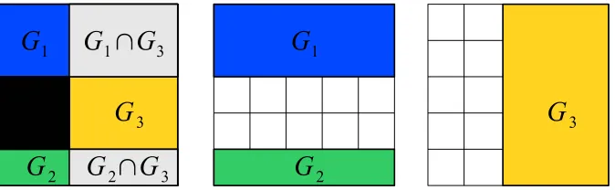
Figure 1: Groups and induced nonzero pattern: three sparsity-inducing groups (middle and right, denoted by_{G1,G2,G3}) with the associated nonzero pattern which is the complement of the union

of groups, that is,(G1∪G2∪G3)c (left, in black).

3. Groups and Sparsity Patterns

We now study the relationship between the normΩdefined in Equation (1) and the nonzero patterns the estimated vector ˆw is allowed to have. We first characterize the set of nonzero patterns, then we provide forward and backward procedures to go back and forth from groups to patterns.

3.1 Stable Patterns Generated by

G

The regularization termΩ(w) =∑_G∈GkdG_{◦wk2is a mixed(ℓ}

1, ℓ2)-norm (Zhao et al., 2009). At the

group level, it behaves like anℓ1-norm and therefore,Ωinduces group sparsity. In other words, each dG

◦w, and equivalently each wG(since the support of dGis exactly G), is encouraged to go to zero.

On the other hand, within the groups G∈

G

, theℓ2-norm does not promote sparsity. Intuitively, for

a certain subset of groups

G

′⊆

G

, the vectors wGassociated with the groups G∈

G

′will be exactly

equal to zero, leading to a set of zeros which is the union of these groups,S_G∈G′G. Thus, the set of

allowed zero patterns should be the union-closure of

G

, that is, (see Figure 1 for an example):

Z

=

[

G∈G′

G;

G

′⊆

G

.

The situation is however slightly more subtle as some zeros can be created by chance (just as reg-ularizing by theℓ2-norm may lead, though it is unlikely, to some zeros). Nevertheless, Theorem 2 shows that, under mild conditions, the previous intuition about the set of zero patterns is correct. Note that instead of considering the set of zero patterns

Z

, it is also convenient to manipulate nonzero patterns, and we define

P

=

\

G∈G′

Gc;

G

′⊆

G

=

Zc; Z_∈

Z

.

We can equivalently use

P

or

Z

by taking the complement of each element of these sets.

second variable and non-vanishing mixed derivative, that is, for any y,y′ inR, _∂∂2ℓ

y′2(y,y′)>0 and ∂2_ℓ

∂y∂y′(y,y′)6=0.

Proposition 1 Let Q denote the Gram matrix 1_n∑n_i=1xix⊤i . We consider the optimization problem

in Equation (2) with µ>0. If Q is invertible or if_{1, . . . ,p_} belongs to

G

, then the problem in Equation (2) admits a unique solution.

Note that the invertibility of the matrix Q requires p_≤n. For high-dimensional settings, the uniqueness of the solution will hold when_{1, . . . ,p_}belongs to

G

, or as further discussed at the end of the proof, as soon as for any j,k_{∈ {}1, . . . ,p_}, there exists a group G_∈

G

which contains both j and k. Adding the group_{1, . . . ,p_}to

G

will in general not modify

P

(and

Z), but it will cause

G

to lose its minimality (in a sense introduced in the next subsection). Furthermore, adding the full group_{1, . . . ,p_}has to be put in parallel with the equivalent (up to the squaring)ℓ2-norm term in the elastic-net penalty (Zou and Hastie, 2005), whose effect is to notably ensure strong convexity. For more sophisticated uniqueness conditions that we have not explored here, we refer the readers to Osborne et al. (2000, Theorem 1, 4 and 5), Rosset et al. (2004, Theorem 5) or Dossal (2007, Theorem 3) in the Lasso case, and Roth and Fischer (2008) for the group Lasso setting. We now turn to the result about the zero patterns of the solution of the problem in Equation (2):

Theorem 2 Assume that Y = (y1, . . . ,yn)⊤is a realization of an absolutely continuous probability

distribution. Let k be the maximal number such that any k rows of the matrix(x1, . . . ,xn)∈Rp×n

are linearly independent. For µ>0, any solution of the problem in Equation (2) with at most k₋1 nonzero coefficients has a zero pattern in

Z

=nS_G∈G′G;

G

′⊆

G

o

almost surely.

In other words, when Y = (y1, . . . ,yn)⊤ is a realization of an absolutely continuous probability

distribution, the sparse solutions have a zero pattern in

Z

=nS_G∈G′G;

G

′⊆

G

o

almost surely. As a corollary of our two results, if the Gram matrix Q is invertible, the problem in Equation (2) has a unique solution, whose zero pattern belongs to

Z

almost surely. Note that with the assumption made on Y , Theorem 2 is not directly applicable to the classification setting. Based on these previous results, we can look at the following usual special cases from Section 2 (we give more examples in Section 3.5):

• ℓ2-norm: the set of allowed nonzero patterns is composed of the empty set and the full set {1, . . . ,p_}.

• ℓ1-norm:

P

is the set of all possible subsets.

• ℓ2-norm andℓ1-norm:

P

is also the set of all possible subsets.

• Group ℓ1-norm:

P

=

Z

is the set of all possible unions of the elements of the partition defining

G

.

• Hierarchical norms: the set of patterns

P

is then all sets J for which all ancestors of elements in J are included in J (Bach, 2008a).

Figure 2:

G

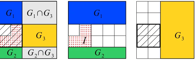
-adapted hull: the pattern of variables I (left and middle, red dotted surface) and its hull (left and right, hatched square) that is defined by the complement of the union of groups that do not intersect I, that is,(G1∪G2∪G3)c.

3.2 General Properties of

G

,

Z

and

P

We now study the different properties of the set of groups

G

and its corresponding sets of patterns

Z

and

P

.

3.2.1 CLOSEDNESS

The set of zero patterns

Z

(respectively, the set of nonzero patterns

P

) is closed under union (re-spectively, intersection), that is, for all K_∈N and all z1, . . . ,zK ∈

Z

, SKk=1zk ∈

Z

(respectively,

p1, . . . ,pK ∈

P

, TKk=1pk∈

P

). This implies that when “reverse-engineering” the set of nonzero

patterns, we have to assume it is closed under intersection. Otherwise, the best we can do is to deal with its intersection-closure. For instance, if we consider a sequence (see Figure 4), we cannot take

P

to be the set of contiguous patterns with length two, since the intersection of such two patterns may result in a singleton (that does not belong to

P

).

3.2.2 MINIMALITY

If a group in

G

is the union of other groups, it may be removed from

G

without changing the sets

Z

or

P

. This is the main argument behind the pruning backward algorithm in Section 3.3. Moreover, this leads to the notion of a minimal set

G

of groups, which is such that for all

G

′⊆

Z

whose union-closure spans

Z, we have

G

⊆

G

′. The existence and uniqueness of a minimal set is a consequence of classical results in set theory (Doignon and Falmagne, 1998). The elements of this minimal set are usually referred to as the atoms of

Z.

Minimal sets of groups are attractive in our setting because they lead to a smaller number of groups and lower computational complexity—for example, for 2 dimensional-grids with rectangu-lar patterns, we have a quadratic possible number of rectangles, that is, _|

Z

|=O(p2), that can be generated by a minimal set

G

whose size is_|

G

|=O(√p).

3.2.3 HULL

Given a set of groups

G

, we can define for any subset I_{⊆ {}1, . . . ,p_}the

G

-adapted hull, or simply hull, as:

Hull(I) =

[

G_∈G,G_∩I=∅ G

c

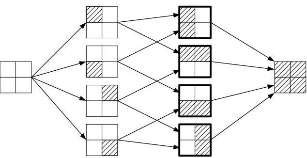
Figure 3: The DAG for the set

Z

associated with the 2_×2-grid. The members of

Z

are the comple-ment of the areas hatched in black. The elecomple-ments of

G

(i.e., the atoms of

Z) are highlighted by bold

edges.

which is the smallest set in

P

containing I (see Figure 2); we always have I_⊆Hull(I)with equality if and only if I_∈

P

. The hull has a clear geometrical interpretation for specific sets

G

of groups. For instance, if the set

G

is formed by all vertical and horizontal half-spaces when the variables are organized in a 2 dimensional-grid (see Figure 5), the hull of a subset I⊂ {1, . . . ,p}is simply the axis-aligned bounding box of I. Similarly, when

G

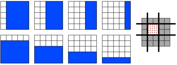
is the set of all half-spaces with all possible orientations (e.g., orientations_±π/4 are shown in Figure 6), the hull becomes the regular convex hull.1 Note that those interpretations of the hull are possible and valid only when we have geomet-rical information at hand about the set of variables.

3.2.4 GRAPHS OFPATTERNS

We consider the directed acyclic graph (DAG) stemming from the Hasse diagram (Cameron, 1994) of the partially ordered set (poset)(G,_⊃). By definition, the nodes of this graph are the elements G of

G

and there is a directed edge from G1 to G2if and only if G1⊃G2and there exists no G∈

G

such that G1⊃G⊃G2(Cameron, 1994). We can also build the corresponding DAG for the set of

zero patterns

Z

⊃

G

, which is a super-DAG of the DAG of groups (see Figure 3 for examples). Note that we obtain also the isomorphic DAG for the nonzero patterns

P

, although it corresponds to the poset(P,_⊂): this DAG will be used in the active set algorithm presented in Section 4.

Prior works with nested groups (Zhao et al., 2009; Bach, 2008a; Kim and Xing, 2010; Jenat-ton et al., 2010a; Schmidt and Murphy, 2010) have also used a similar DAG structure, with the slight difference that in these works, the corresponding hierarchy of variables is built from the prior knowledge about the problem at hand (e.g., the tree of wavelets in Zhao et al., 2009, the decom-position of kernels in Bach, 2008a or the hierarchy of genes in Kim and Xing, 2010). The DAG we introduce here on the set of groups naturally and always comes up, with no assumption on the variables themselves (for which no DAG is defined in general).

3.3 From Patterns to Groups

We now assume that we want to impose a priori knowledge on the sparsity structure of a solution ˆ

w of our regularized problem in Equation (2). This information can be exploited by restricting the patterns allowed by the normΩ. Namely, from an intersection-closed set of zero patterns

Z

, we can build back a minimal set of groups

G

by iteratively pruning away in the DAG corresponding to

Z,

all sets which are unions of their parents. See Algorithm 1. This algorithm can be found under a different form in Doignon and Falmagne (1998)—we present it through a pruning algorithm on the DAG, which is natural in our context (the proof of the minimality of the procedure can be found in Appendix C). The complexity of Algorithm 1 is O(p_|

Z

|2_{). The pruning may reduce significantly the}

number of groups necessary to generate the whole set of zero patterns, sometimes from exponential in p to polynomial in p (e.g., theℓ1-norm). In Section 3.5, we give other examples of interest where |

G

|(and_|

P

|) is also polynomial in p.

Algorithm 1 Backward procedure

Input: Intersection-closed family of nonzero patterns

P

.

Output: Set of groups

G

.

Initialization: Compute

Z

=_{Pc; P_∈

P

}and set

G

=

Z

. Build the Hasse diagram for the poset(Z,_⊃).

for t=minG_∈Z|G|to maxG_∈Z|G|do

for each node G_∈

Z

such that_|G_|=t do

if S_{C∈Children(G)}C=G then if (Parents(G)₆=∅) then

Connect children of G to parents of G.

end if

Remove G from

G

.

end if end for end for

3.4 From Groups to Patterns

The forward procedure presented in Algorithm 2, taken from Doignon and Falmagne (1998), allows the construction of

Z

from

G

. It iteratively builds the collection of patterns by taking unions, and has complexity O(p_|

Z

||

G

|2_{). The general scheme is straightforward. Namely, by considering}

Algorithm 2 Forward procedure

Input: Set of groups

G

=_{G1, . . . ,GM}.

Output: Collection of zero patterns

Z

and nonzero patterns

P

.

Initialization:

Z

=_{∅}.

for m=1 to M do C=_{∅}

for each Z_∈

Z

do

if(Gm*Z) and (∀G∈{G1, . . . ,Gm−1}, G⊆Z∪Gm⇒G⊆Z)then

C_←C_{∪ {}Z_∪Gm}. end if

end for

Z

←

Z

∪C.

end for

P

=_{Zc; Z_∈

Z

}.

3.5 Examples

We now present several examples of sets of groups

G

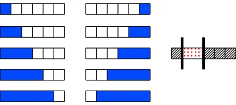
, especially suited to encode geometric and temporal prior information.

3.5.1 SEQUENCES

Given p variables organized in a sequence, if we want only contiguous nonzero patterns, the back-ward algorithm will lead to the set of groups which are intervals[1,k]k_∈{1,...,p₋1_}and[k,p]k_∈{2,...,p_},

with both |

Z

|=O(p2) and |

G

|=O(p) (see Figure 4). Imposing the contiguity of the nonzero patterns is for instance relevant for the diagnosis of tumors, based on the profiles of arrayCGH (Rapaport et al., 2008).

Figure 4: (Left and middle) The set of groups (blue areas) to penalize in order to select contiguous patterns in a sequence. (Right) An example of such a nonzero pattern (red dotted area) with its corresponding zero pattern (hatched area).

3.5.2 TWO-DIMENSIONALGRIDS

and |

G

|=O(√p). This type of structure is encountered in object or scene recognition, where the selected rectangle would correspond to a certain box inside an image, that concentrates the predictive power for a given class of object/scene (Harzallah et al., 2009).

Larger set of convex patterns can be obtained by adding in

G

half-planes with other orienta-tions than vertical and horizontal. For instance, if we use planes with angles that are multiples of

π/4, the nonzero patterns of

P

can have polygonal shapes with up to 8 faces. In this sense, if we keep on adding half-planes with finer orientations, the nonzero patterns of

P

can be described by polygonal shapes with an increasingly larger number of faces. The standard notion of convexity defined inR2would correspond to the situation where an infinite number of orientations is consid-ered (Soille, 2003). See Figure 6. The number of groups is linear in √p with constant growing linearly with the number of angles, while_|

Z

|grows more rapidly (typically non-polynomially in the number of angles). Imposing such convex-like regions turns out to be useful in computer vision. For instance, in face recognition, it enables the design of localized features that improve upon the robustness to occlusions (Jenatton et al., 2010b). In the same vein, regularizations with similar two-dimensional sets of groups have led to good performances in background subtraction tasks (Mairal et al., 2010b), where the pixel spatial information is crucial to avoid scattered results. Another ap-plication worth being mentioned is the design of topographic dictionaries in the context of image processing (Kavukcuoglu et al., 2009; Mairal et al., 2011). In this case, dictionaries self-organize and adapt to the underlying geometrical structure encoded by the two-dimensional set of groups.

Figure 5: Vertical and horizontal groups: (Left) the set of groups (blue areas) with their (not dis-played) complements to penalize in order to select rectangles. (Right) An example of nonzero pat-tern (red dotted area) recovered in this setting, with its corresponding zero patpat-tern (hatched area).

3.5.3 EXTENSIONS

The sets of groups presented above can be straightforwardly extended to more complicated topolo-gies, such as three-dimensional spaces discretized in cubes or spherical volumes discretized in slices. Similar properties hold for such settings. For instance, if all the axis-aligned half-spaces are considered for

G

in a three-dimensional space, then

P

is the set of all possible rectangular boxes with_|

P

|=O(p2_)and|

_G

_|=O(p1/3_{). Such three-dimensional structures are interesting to retrieve}

Figure 6: Groups with _±π/4 orientations: (Left) the set of groups (blue areas) with their (not displayed) complements to penalize in order to select diamond-shaped patterns. (Right) An example of nonzero pattern (red dotted area) recovered in this setting, with its corresponding zero pattern (hatched area).

groups, embedded in the three-dimensional space obtained by tracking the frames over time. Finally, in the context of matrix-based optimization problems, for example, multi-task learning and dictio-nary learning, sets of groups

G

can also be designed to encode structural constraints the solutions must respect. This notably encompasses banded structures (Levina et al., 2008) and simultaneous row/column sparsity for CUR matrix factorization (Mairal et al., 2011).

3.5.4 REPRESENTATION ANDCOMPUTATION OF

G

The sets of groups described so far can actually be represented in a same form, that lends itself well to the analysis of the next section. When dealing with a discrete sequence of length l (see Figure 4), we have

G

= _{gk₋; k_{∈ {}1, . . . ,l₋1_{}} ∪ {}gk₊; k_{∈ {}2, . . . ,l_}},

=

G

left∪

G

right,

with gk₋ =_{i; 1≤i≤k} and gk₊ =_{i; l ≥i≥k}. In other words, the set of groups

G

can be rewritten as a partition2in two sets of nested groups,

G

leftand

G

right.

The same goes for a two-dimensional grid, with dimensions h_×l (see Figure 5 and Figure 6). In this case, the nested groups we consider are defined based on the following groups of variables

gk,θ=_{(i,j)_{∈ {}1, . . . ,l_{} × {}1, . . . ,h_}; cos(θ)i+sin(θ)j_≤k_},

where k_∈Zis taken in an appropriate range. The nested groups we obtain in this way are therefore parameterized by an angle3θ,θ_∈(₋π;π]. We refer to this angle as an orientation, since it defines the normal vector cos_sin(θ)(θ) to the line {(i,j)_∈R2_{; cos(}θ_)i+sin(θ_{)j=k}. In the example of the}

rectangular groups (see Figure 5), we have four orientations, with θ_{∈ {}0,π/2,₋π/2,π_}. More generally, if we denote byΘthe set of the orientations, we have

G

= [

θ∈Θ

G

θ,

2. Note the subtlety: the setsGθare disjoint, that isGθ∩Gθ′=∅forθ6=θ′, but groups inG_θandG_θ′can overlap.

whereθ∈Θindexes the partition of

G

in sets

G

θof nested groups of variables. Although we have not detailed the case ofR3, we likewise end up with a similar partition of

G

.

4. Optimization and Active Set Algorithm

For moderate values of p, one may obtain a solution for Problem (2) using generic toolboxes for second-order cone programming (SOCP) whose time complexity is equal to O(p3.5+_|

G

|3.5_)(Boyd

and Vandenberghe, 2004), which is not appropriate when p or_|

G

|are large. This time complexity corresponds to the computation of a solution of Problem (2) for a single value of the regularization parameter µ.

We present in this section an active set algorithm (Algorithm 3) that finds a solution for Prob-lem (2) by considering increasingly larger active sets and checking global optimality at each step. When the rectangular groups are used, the total complexity of this method is in O(s max_{p1.75,s3.5_}), where s is the size of the active set at the end of the optimization. Here, the sparsity prior is exploited for computational advantages. Our active set algorithm needs an underlying black-box SOCP solver; in this paper, we consider both a first order approach (see Appendix H) and a SOCP method4—in our experiments, we useSDPT3(Toh et al., 1999; T¨ut¨unc¨u et al., 2003). Our active set algorithm extends to general overlapping groups the work of Bach (2008a), by further assuming that it is computationally possible to have a time complexity polynomial in the number of variables p.

We primarily focus here on finding an efficient active set algorithm; we defer to future work the design of specific SOCP solvers, for example, based on proximal techniques (see, e.g., Nesterov, 2007; Beck and Teboulle, 2009; Combettes and Pesquet, 2010, and numerous references therein), adapted to such non-smooth sparsity-inducing penalties.

4.1 Optimality Conditions: From Reduced Problems to Full Problems

It is simpler to derive the algorithm for the following regularized optimization problem5which has the same solution set as the regularized problem of Equation (2) when µ andλare allowed to vary (Borwein and Lewis, 2006, see Section 3.2):

min

w∈Rp 1 n

n

∑

i=1

ℓ yi,w⊤xi

+λ 2[Ω(w)]

2_{. (3)}

In active set methods, the set of nonzero variables, denoted by J, is built incrementally, and the problem is solved only for this reduced set of variables, adding the constraint wJc =0 to Equa-tion (3). In the subsequent analysis, we will use arguments based on duality to monitor the optimal-ity of our active set algorithm. We denote by L(w) =1

n∑ n

i=1ℓ yi,w⊤xi

the empirical risk (which is by assumption convex and continuously differentiable) and by L∗its Fenchel-conjugate, defined as (Boyd and Vandenberghe, 2004; Borwein and Lewis, 2006):

L∗(u) = sup

w∈Rp{

w⊤u₋L(w)_}.

4. The C++/Matlab code used in the experiments may be downloaded from the authors website.

5. It is also possible to derive the active set algorithm for the constrained formulation minw_∈Rp1_n∑n_i=1ℓy_i,w⊤x_i such that Ω(w)≤λ. However, we empirically found it more difficult to select

The restriction of L to R|J| is denoted LJ(wJ) =L(w)˜ for ˜wJ =wJ and ˜wJc =0, with Fenchel-conjugate L∗_J. Note that, as opposed to L, we do not have in general L∗_J(κJ) =L∗(κ˜)for ˜κJ=κJand

˜

κJc=0.

For a potential active set J_{⊂ {}1, . . . ,p_}which belongs to the set of allowed nonzero patterns

P

, we denote by

G

Jthe set of active groups, that is, the set of groups G∈

G

such that G∩J6=∅. We

consider the reduced normΩJdefined onR|J|as

ΩJ(wJ) =

∑

G∈G

kdG

J ◦wJk2=

∑

G∈GJ

kdG

J◦wJk2,

and its dual normΩ∗_J(κJ) =maxΩJ(wJ)≤1w⊤JκJ, also defined onR|J|. The next proposition (see proof

in Appendix D) gives the optimization problem dual to the reduced problem (Equation (4) below):

Proposition 3 (Dual Problems) Let J_{⊆ {}1, . . . ,p_}. The following two problems

min

wJ∈R|J|

LJ(wJ) +

λ

2[ΩJ(wJ)]

2_{, (4)}

max κJ∈R|J| −L

∗

J(−κJ)−

1 2λ[Ω

∗

J(κJ)]2,

are dual to each other and strong duality holds. The pair of primal-dual variables _{wJ,κJ} is

optimal if and only if we have

(

κJ =−∇LJ(wJ),

w⊤_JκJ =_λ1[Ω∗J(κJ)]2=λ[ΩJ(wJ)]2.

As a brief reminder, the duality gap of a minimization problem is defined as the difference between the primal and dual objective functions, evaluated for a feasible pair of primal/dual variables (Boyd and Vandenberghe, 2004, see Section 5.5). This gap serves as a certificate of (sub)optimality: if it is equal to zero, then the optimum is reached, and provided that strong duality holds, the converse is true as well (Boyd and Vandenberghe, 2004, see Section 5.5).

The previous proposition enables us to derive the duality gap for the optimization Problem (4), that is reduced to the active set of variables J. In practice, this duality gap will always vanish (up to the precision of the underlying SOCP solver), since we will sequentially solve Problem (4) for increasingly larger active sets J. We now study how, starting from the optimality of the problem in Equation (4), we can control the optimality, or equivalently the duality gap, for the full problem in Equation (3). More precisely, the duality gap of the optimization problem in Equation (4) is

LJ(wJ) +L∗J(−κJ) +

λ

2[ΩJ(wJ)]

2

+ 1

2λ[Ω ∗

J(κJ)]2

= nLJ(wJ) +L∗J(−κJ) +w⊤JκJ o

+ λ

2[ΩJ(wJ)]

2

+ 1 2λ[Ω

∗

J(κJ)]2−w⊤JκJ

,

relative to LJ andΩJ. Thus, if we have a primal candidate wJ and we chooseκJ=−∇LJ(wJ), the

duality gap relative to LJvanishes and the total duality gap then reduces to

λ

2[ΩJ(wJ)]

2

+ 1

2λ[Ω ∗

J(κJ)]2−w⊤JκJ.

In order to check that the reduced solution wJis optimal for the full problem in Equation (3), we

pad wJwith zeros on Jcto define w and computeκ=−∇L(w), which is such thatκJ=−∇LJ(wJ).

For our given candidate pair of primal/dual variables_{w,κ_}, we then get a duality gap for the full problem in Equation (3) equal to

λ

2[Ω(w)]

2₊ 1

2λ[Ω ∗_(κ)]2

−w⊤κ

= λ

2[Ω(w)]

2₊ 1

2λ[Ω ∗_(κ)]2

−w⊤_JκJ

= λ

2[Ω(w)]

2

+ 1 2λ[Ω

∗_(κ)]2

−λ₂[ΩJ(wJ)]2−

1 2λ[Ω

∗

J(κJ)]2

= 1

2λ

[Ω∗(κ)]2₋[Ω∗_J(κJ)]2

= 1

2λ

[Ω∗(κ)]2₋λw⊤_JκJ

.

Computing this gap requires computing the dual norm which itself is as hard as the original problem, prompting the need for upper and lower bounds onΩ∗(see Propositions 4 and 5 for more details).

Figure 8: The active set (black) and the candidate patterns of variables, that is, the variables in K_\J (hatched in black) that can become active. The groups in red are those inSK_∈Π_P(J)

G

K\

G

J, while

the blue dotted group is in

F

J\(SK∈ΠP(J)

G

K\

G

J). The blue dotted group does not intersect with

any patterns inΠ_P(J).

4.2 Active Set Algorithm

We can interpret the active set algorithm as a walk through the DAG of nonzero patterns allowed by the normΩ. The parentsΠP(J)of J in this DAG are exactly the patterns containing the variables that may enter the active set at the next iteration of Algorithm 3. The groups that are exactly at the boundaries of the active set (referred to as the fringe groups) are

F

J ={G∈(GJ)c ; ∄G′ ∈

(GJ)c,G⊆G′}, that is, the groups that are not contained by any other inactive groups.

In simple settings, for example, when

G

is the set of rectangular groups, the correspondence between groups and variables is straightforward since we have

F

J=SK∈ΠP(J)

G

K\

G

J(see Figure 7).

However, in general, we just have the inclusion(S_K∈ΠP(J)

G

K\

G

J)⊆

F

J and some elements of

F

J

might not correspond to any patterns of variables inΠP(J)(see Figure 8).

We now present the optimality conditions (see proofs in Appendix E) that monitor the progress of Algorithm 3:

Proposition 4 (Necessary condition) If w is optimal for the full problem in Equation (3), then

max

K∈ΠP(J)

∇L(w)_K\J

2

∑H∈GK\GJ dH_K\J

_∞

≤

−λw⊤∇L(w) 12_{. (N)}

Proposition 5 (Sufficient condition) If

max

G∈FJ (

∑

k∈G

∇

L(w)k

∑H_∋k,H_∈(GJ)cd_kH 2)

1 2

≤λ

(2ε₋w⊤∇L(w)) 12_{, (S} ε)

Note that for the Lasso, the conditions(N)and(S0)(i.e., the sufficient condition taken withε=

0) are both equivalent (up to the squaring ofΩ) to the condition_k∇L(w)Jck∞≤ −w⊤∇L(w), which is the usual optimality condition (Fuchs, 2005; Tibshirani, 1996; Wainwright, 2009). Moreover, when they are not satisfied, our two conditions provide good heuristics for choosing which K∈ΠP(J) should enter the active set.

More precisely, since the necessary condition (N) directly deals with the variables (as opposed to groups) that can become active at the next step of Algorithm 3, it suffices to choose the pattern K_∈

ΠP(J)that violates most the condition.

The heuristics for the sufficient condition (Sε) implies that, to go from groups to variables, we simply consider the group G_∈

F

J violating the sufficient condition the most and then take all the

patterns of variables K_∈Π_P(J)such that K_∩G₆=∅to enter the active set. If G_∩(S_K∈ΠP(J)K) =

∅, we look at all the groups H∈

F

J such that H∩G6=∅and apply the scheme described before

(see Algorithm 4).

A direct consequence of this heuristics is that it is possible for the algorithm to jump over the right active set and to consider instead a (slightly) larger active set as optimal. However if the active set is larger than the optimal set, then (it can be proved that) the sufficient condition(S0)is satisfied,

and the reduced problem, which we solve exactly, will still output the correct nonzero pattern. Moreover, it is worthwhile to notice that in Algorithm 3, the active set may sometimes be in-creased only to make sure that the current solution is optimal (we only check a sufficient condition of optimality).

Algorithm 3 Active set algorithm

Input: Data{(xi,yi), i=1, . . . ,n}, regularization parameterλ,

Duality gap precisionε, maximum number of variables s.

Output: Active set J, loading vector ˆw.

Initialization: J=_{∅}, ˆw=0.

while (N)is not satisfiedand _|J_{| ≤}s do

Replace J by violating K_∈Π_P(J)in (N).

Solve the reduced problem min_wJ∈R|J|LJ(wJ) +λ₂[ΩJ(wJ)]2 to get ˆw. end while

while (S_ε)is not satisfiedand _|J_{| ≤}s do

Update J according to Algorithm 4.

Solve the reduced problem min_wJ∈R|J|LJ(wJ) +λ₂[ΩJ(wJ)]2 to get ˆw. end while

4.2.1 CONVERGENCE OF THEACTIVESETALGORITHM

The procedure described in Algorithm 3 can terminate in two different states. If the procedure stops because of the limit on the number of active variables s, the solution might be suboptimal. Note that, in any case, we have at our disposal a upper-bound on the duality gap.

Algorithm 4 Heuristics for the sufficient condition (Sε) Let G_∈

F

J be the group that violates (Sε) most. if (G_∩(S_K∈ΠP(J)K)₆=∅) then

for K_∈ΠP(J)such that K∩G6=∅do J_←J_∪K.

end for else

for H_∈

F

J such that H∩G6=∅do for K∈ΠP(J)such that K∩H6=∅do

J_←J_∪K.

end for end for end if

4.2.2 ALGORITHMICCOMPLEXITY

We analyze in detail the time complexity of the active set algorithm when we consider sets of groups

G

such as those presented in the examples of Section 3.5. We recall that we denote byΘthe set of orientations in

G

(for more details, see Section 3.5). For such choices of

G

, the fringe groups

F

J

reduces to the largest groups of each orientation and therefore_|

F

J| ≤ |Θ|. We further assume that

the groups in

G

θare sorted by cardinality, so that computing

F

Jcosts O(|Θ|).

Given an active set J, both the necessary and sufficient conditions require to have access to the direct parentsΠ_P(J)of J in the DAG of nonzero patterns. In simple settings, for example, when

G

is the set of rectangular groups, this operation can be performed in O(1)(it just corresponds to scan the (up to) four patterns at the edges of the current rectangular hull).

However, for more general orientations, computingΠ_P(J)requires to find the smallest nonzero patterns that we can generate from the groups in

F

J, reduced to the stripe of variables around the

current hull. This stripe of variables can be computed asS_G∈(GJ)c_\F JG

c

\J, so that gettingΠP(J) costs O(s2|Θ|_+p|

_G

_{|)in total.}

Thus, if the number of active variables is upper bounded by s≪p (which is true if our target is actually sparse), the time complexity of Algorithm 3 is the sum of:

• the computation of the gradient, O(snp)for the square loss.

• if the underlying solver called upon by the active set algorithm is a standard SOCP solver, O(s maxJ∈P,|J|≤s|

G

J|3.5+s4.5)(note that the term s4.5could be improved upon by using

warm-restart strategies for the sequence of reduced problems).

• t1times the computation of(N), that is O(t1(s2|Θ|+p|

G

|+sn2_θ) +p|

G

|) =O(t1p|

G

|).

During the initialization (i.e., J=∅), we have_|Π_P(∅)_|=O(p)(since we can start with any singletons), and_|

G

K\

G

J|=|

G

K|=|

G

|, which leads to a complexity of O(p|

G

|)for the sum

∑G∈GK\GJ =∑G∈GK. Note however that this sum does not depend on J and can therefore be cached if we need to make several runs with the same set of groups

G

.

• t2times the computation of(Sε), that is O(t2(s2|Θ|+p|

G

|+|Θ|2+|Θ|p+p|

G

|)) =O(t2p|

G

|),

We finally get complexity with a leading term in O(sp_|

G

|+s maxJ∈P,|J|≤s|

G

J|3.5+s4.5), which

is much better than O(p3.5_+|

_G

_|3.5_{), without an active set method. In the example of the}

two-dimensional grid (see Section 3.5), we have_|

G

|=O(√p)and O(s max_{p1.75,s3.5_}) as total com-plexity. The simulations of Section 6 confirm that the active set strategy is indeed useful when s is much smaller than p. Moreover, the two extreme cases where s_≈p or p_≪1 are also shown not to be advantageous for the active set strategy, since either it is cheaper to use the SOCP solver directly on the p variables, or we uselessly pay the additional fixed-cost of the active set machinery (such as computing the optimality conditions). Note that we have derived here the theoretical complexity of the active set algorithm when we use an interior point method as underlying solver. With the first order method presented in Appendix H, we would instead get a total complexity in O(sp1.5_). 4.3 Intersecting Nonzero Patterns

We have seen so far how overlapping groups can encore prior information about a desired set of (non)zero patterns. In practice, controlling these overlaps may be delicate and hinges on the choice of the weights(dG₎

G_∈G (see the experiments in Section 6). In particular, the weights have to take into account that some variables belonging to several overlapping groups are penalized multiple times.

However, it is possible to keep the benefit of overlapping groups whilst limiting their side effects, by taking up the idea of support intersection (Bach, 2008c; Meinshausen and B¨uhlmann, 2010). First introduced to stabilize the set of variables recovered by the Lasso, we reuse this technique in a different context, based on the fact that

Z

is closed under union.

If we deal with the same sets of groups as those considered in Section 3.5, it is natural to rewrite

G

as S_θ∈Θ

G

θ, where Θ is the set of the orientations of the groups in

G

(for more details, see Section 3.5). Let us denote by ˆw and ˆwθthe solutions of Problem (3), where the regularization term

Ωis respectively defined by the groups in

G

and by the groups6in

G

θ.

The main point is that, since

P

is closed under intersection, the two procedures described below actually lead to the same set of allowed nonzero patterns:

a) Simply considering the nonzero pattern of ˆw.

b) Taking the intersection of the nonzero patterns obtained for each ˆwθ,θinΘ.

With the latter procedure, although the learning of several models ˆwθ is required (a number of times equals to the number of orientations considered, for example, 2 for the sequence, 4 for the rectangular groups and more generally_|Θ_|times), each of those learning tasks involves a smaller number of groups (that is, just the ones belonging to

G

θ). In addition, this procedure is a variable selection technique that therefore needs a second step for estimating the loadings (restricted to the selected nonzero pattern). In the experiments, we follow Bach (2008c) and we use an ordinary least squares (OLS). The simulations of Section 6 will show the benefits of this variable selection approach.

5. Pattern Consistency

In this section, we analyze the model consistency of the solution of the problem in Equation (2) for the square loss. Considering the set of nonzero patterns

P

derived in Section 3, we can only hope to estimate the correct hull of the generating sparsity pattern, since Theorem 2 states that other patterns occur with zero probability. We derive necessary and sufficient conditions for model consistency in a low-dimensional setting, and then consider a high-dimensional result.

We consider the square loss and a fixed-design analysis (i.e., x1, . . . ,xnare fixed). The extension

of the following consistency results to other loss functions is beyond the scope of the paper (see for instance Bach, 2009). We assume that for all i_{∈ {}1, . . . ,n_}, yi =w⊤xi+εi where the vector

εis an i.i.d. vector with Gaussian distributions with mean zero and variance σ2>0, and w_∈Rp is the population sparse vector; we denote by J the

G

-adapted hull of its nonzero pattern. Note that estimating the

G

-adapted hull of w is equivalent to estimating the nonzero pattern of w if and only if this nonzero pattern belongs to

P

. This happens when our prior information has led us to consider an appropriate set of groups

G

. Conversely, if

G

is misspecified, recovering the hull of the nonzero pattern of w may be irrelevant, which is for instance the case if w= w1

0

∈R2 _and

G

=_{{1_},_{1,2_}}. Finding the appropriate structure of

G

directly from the data would therefore be interesting future work.

5.1 Consistency Condition

We begin with the low-dimensional setting where n is tending to infinity with p fixed. In addition, we also assume that the design is fixed and that the Gram matrix Q=1_n∑n_i=1xix⊤i is invertible with

positive-definite (i.e., invertible) limit: limn→∞Q=Q≻0. In this setting, the noise is the only source of randomness. We denote by rJthe vector defined as

∀j_∈J, rj=wj

∑

G∈GJ,G∋j

(dG

j)2kd

G

◦w_k−₂1

.

In the Lasso and group Lasso setting, the vector rJis respectively the sign vector sign(wJ)and the vector defined by the blocks( wG

kwGk2)G∈GJ. We define Ωc_J(wJc) =∑_G∈(G

J)c

d_JGc◦wJc

2 (which is the norm composed of inactive groups)

with its dual norm(Ωc

J)∗; note the difference with the norm reduced to Jc, defined asΩJc(w_Jc) =

∑G∈G

dG_Jc◦wJc

2.

The following Theorem gives the sufficient and necessary conditions under which the hull of the generating pattern is consistently estimated. Those conditions naturally extend the results of Zhao and Yu (2006) and Bach (2008b) for the Lasso and the group Lasso respectively (see proof in Appendix F).

Theorem 6 (Consistency condition) Assume µ_→0, µ√n_→∞in Equation (2). If the hull is con-sistently estimated, then(Ωc

J)∗[QJcJQ−

1

JJrJ]≤1. Conversely, if(ΩJc)∗[QJcJQ−

1

JJrJ]<1, then the hull is consistently estimated, that is,

P(_{j_{∈ {}1, . . . ,p_},wˆj6=0}=J) −→ n→+∞1.

The two previous propositions bring into play the dual norm(Ωc

Equation (3). However, we can prove bounds similar to those obtained in Propositions 4 and 5 for the necessary and sufficient conditions.

5.1.1 COMPARISON WITH THELASSO ANDGROUPLASSO

For theℓ1-norm, our two bounds lead to the usual consistency conditions for the Lasso, that is, the quantity_kQJc_JQ−1

JJsign(wJ)k∞ must be less or strictly less than one. Similarly, when

G

defines a partition of_{1, . . . ,p_}and if all the weights equal one, our two bounds lead in turn to the consistency conditions for the group Lasso, that is, the quantity maxG∈(GJ)ckQG Hull(J)Q

−1

Hull(J)Hull(J)( w G

kwGk2)G∈GJk2 must be less or strictly less than one.

5.2 High-Dimensional Analysis

We prove a high-dimensional variable consistency result (see proof in Appendix G) that extends the corresponding result for the Lasso (Zhao and Yu, 2006; Wainwright, 2009), by assuming that the consistency condition in Theorem 6 is satisfied.

Theorem 7 Assume that Q has unit diagonal, κ=λmin(QJJ)>0 and(ΩcJ)∗[QJc_JQ−1

JJrJ]<1−τ, with τ>0. If τµ√n_≥σC3(G,J), and µ|J|1/2 ≤C4(G,J),then the probability of incorrect hull

selection is upper bounded by:

exp

−nµ 2τ2_C

1(G,J)

2σ2

+2_|J_|exp

−nC₂2(G,J) |J_|σ2

,

where C1(G,J), C2(G,J), C3(G,J) and C4(G,J) are constants defined in Appendix G, which

es-sentially depend on the groups, the smallest nonzero coefficient of w and how close the support

{j_∈J : wj6=0}of w is to its hull J, that is the relevance of the prior information encoded by

G

.

In the Lasso case, we have C1(G,J) =O(1), C2(G,J) =O(|J|−2), C3(G,J) =O((log p)1/2)and

C4(G,J) =O(|J|−1), leading to the usual scaling n≈log p and µ≈σ(log p/n)1/2.

We can also give the scaling of these constants in simple settings where groups overlap. For instance, let us consider that the variables are organized in a sequence (see Figure 4). Let us further assume that the weights(dG₎

G∈G satisfy the following two properties:

a) The weights take into account the overlaps, that is,

dG

j =β(|{H∈

G

; H∋ j, H⊂G and H6=G}|),

with t_7→β(t)_∈(0,1]a non-increasing function such thatβ(0) =1,

b) The term

max

j∈{1,...,p}_G∋

∑

_j,G∈Gd G

j

is upper bounded by a constant

K

independent of p.

Note that we consider such weights in the experiments (see Section 6). Based on these assumptions, some algebra directly leads to

We thus obtain a scaling similar to the Lasso (with, in addition, a control of the allowed nonzero patterns). With stronger assumptions on the possible positions of J, we may have better scalings, but these are problem-dependent (a careful analysis of the group-dependent constants would still be needed in all cases).

6. Experiments

In this section, we carry out several experiments to illustrate the behavior of the sparsity-inducing normΩ. We denote by Structured-lasso, or simply Slasso, the models regularized by the normΩ. In addition, the procedure (introduced in Section 4.3) that consists in intersecting the nonzero patterns obtained for different models of Slasso will be referred to as Intersected Structured-lasso, or simply ISlasso.

Throughout the experiments, we consider noisy linear models Y =X w+ε, where w_∈Rpis the generating loading vector andεis a standard Gaussian noise vector with its variance set to satisfy

kX w_k2=3_kε_k2. This consequently leads to a fixed signal-to-noise ratio. We assume that the vector

w is sparse, that is, it has only a few nonzero components, that is,_|J_{| ≪}p. We further assume that these nonzero components are either organized on a sequence or on a two-dimensional grid (see Figure 9). Moreover, we consider sets of groups

G

such as those presented in Section 3.5. We also consider different choices for the weights(dG₎

G∈G that we denote by (W1), (W2) and (W3) (we will keep this notation throughout the following experiments):

(W1): Uniform weights, dG

j =1,

(W2): Weights depending on the size of the groups, dG

j =|G|−2, (W3): Weights for overlapping groups, dG

j =ρ|{H∈G; H∋j,H⊂GandH6=G}|,for someρ∈(0,1).

For each orientation in

G

, the third type of weights (W3) aims at reducing the unbalance caused by the overlapping groups. Specifically, given a group G_∈

G

and a variable j_∈G, the corresponding weight dG

j is all the more small as the variable j already belongs to other groups with the same

orientation. Unless otherwise specified, we use the third type of weights (W3) with ρ=0.5. In the following experiments, the loadings wJ, as well as the design matrices, are generated from a standard Gaussian distribution with identity covariance matrix. The positions of J are also random and are uniformly drawn.

6.1 Consistent Hull Estimation

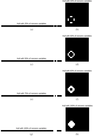
We first illustrate Theorem 6 that establishes necessary and sufficient conditions for consistent hull estimation. To this end, we compute the probability of correct hull estimation when we consider diamond-shaped generating patterns of_|J_|=24 variables on a 20_×20-dimensional grid (see Fig-ure 9h). Specifically, we generate 500 covariance matrices Q distributed according to a Wishart distribution withδdegrees of freedom, whereδis uniformly drawn in_{1,2, . . . ,10p_}.7 The diago-nal terms of Q are then re-normalized to one. For each of these covariance matrices, we compute an

Hull with 25% of nonzero variables

(a) (b)

Hull with 50% of nonzero variables

(c)

Hull with 50% of nonzero variables

(d)

Hull with 75% of nonzero variables

(e)

Hull with 83% of nonzero variables

(f)

Hull with 100% of nonzero variables

(g)

Hull with 100% of nonzero variables

(h)

−0.50 0 0.5 0.2

0.4 0.6 0.8 1

log

10(Consistency condition)

Pattern recovery probability

Figure 10: Consistent hull estimation: probability of correct hull estimation versus the consistency condition(Ωc

J)∗[QJc_JQ−1

JJrJ]. The transition appears at zero, in good agreement with Theorem 6.

entire regularization path based on one realization of_{J,w,X,ε_}, with n=3000 samples. The quan-tities_{J,w,ε_}are generated as described previously, while the n rows of X are Gaussian with co-variance Q. After repeating 20 times this computation for each Q, we eventually report in Figure 10 the probabilities of correct hull estimation versus the consistency condition(Ωc

J)∗[QJc_JQ−1 JJrJ]. In good agreement with Theorem 6, comparing(Ωc

J)∗[QJcJQ−

1

JJrJ]to 1 determines whether the hull is consistently estimated.

6.2 Structured Variable Selection

We show in this experiment that the prior information we put through the normΩimproves upon the ability of the model to recover spatially structured nonzero patterns. We are looking at two situations where we can express such a prior throughΩ, namely (1) the selection of a contiguous pattern on a sequence (see Figure 9g) and (2) the selection of a convex pattern on a grid (see Figure 9h).

In what follows, we consider p=400 variables with generating patterns w whose hulls are composed of_|J_|=24 variables. For different sample sizes n_{∈ {}100,200,300,400,500,700,1000_}, we consider the probabilities of correct recovery and the (normalized) Hamming distance to the true nonzero patterns. For the realization of a random setting_{J,w,X,ε_}, we compute an entire regularization path over which we collect the closest Hamming distance to the true nonzero pattern and whether it has been exactly recovered for some µ. After repeating 50 times this computation for each sample size n, we report the results in Figure 11.

First and foremost, the simulations highlight how important the weights(dG₎

G∈G are. In partic-ular, the uniform (W1) and size-dependent weights (W2) perform poorly since they do not take into account the overlapping groups. The models learned with such weights do not manage to recover the correct nonzero patterns (in that case, the best model found on the path corresponds to the empty solution, with a normalized Hamming distance of_|J_|/p=0.06—see Figure 11c).

Although groups that moderately overlap do help (e.g., see Slasso with the weights (W3) on Figure 11c), it remains delicate to handle groups with many overlaps, even with an appropriate choice of(dG₎

100 200 300 400 500 700 1000 0

0.2 0.4 0.6 0.8 1 1.2 1.4

Sample size

Pattern recovery probability

Lasso Slasso − W1 Slasso − W2 Slasso − W3 ISlasso − W3

(a) Probability of recovery for the sequence

100 200 300 400 500 700 1000

0 0.2 0.4 0.6 0.8 1 1.2 1.4

Sample size

Pattern recovery probability

Lasso Slasso − W3 ISlasso − W3 ISlasso − W3 (π/4)

(b) Probability of recovery for the grid

100 200 300 400 500 700 1000

0 0.01 0.02 0.03 0.04 0.05 0.06 0.07

Sample size

Pattern recovery error

Lasso Slasso − W1 Slasso − W2 Slasso − W3 ISlasso − W3

(c) Distance to the true pattern for the sequence

100 200 300 400 500 700 1000

0 0.01 0.02 0.03 0.04 0.05 0.06 0.07

Sample size

Pattern recovery error

Lasso Slasso − W3 ISlasso − W3 ISlasso − W3 (π/4)

(d) Distance to the true pattern for the grid