Efficient Algorithms for Decision Tree Cross-validation
Hendrik Blockeel [email protected]
Jan Struyf [email protected]
Department of Computer Science Katholieke Universiteit Leuven
Celestijnenlaan 200A, B-3001 Leuven, Belgium
Editors: Carla E. Brodley and Andrea Danyluk
Abstract
Cross-validation is a useful and generally applicable technique often employed in machine learn-ing, including decision tree induction. An important disadvantage of straightforward implemen-tation of the technique is its compuimplemen-tational overhead. In this paper we show that, for decision trees, the computational overhead of cross-validation can be reduced significantly by integrating the cross-validation with the normal decision tree induction process. We discuss how existing de-cision tree algorithms can be adapted to this aim, and provide an analysis of the speedups these adaptations may yield. We identify a number of parameters that influence the obtainable speedups, and validate and refine our analysis with experiments on a variety of data sets with two different im-plementations. Besides cross-validation, we also briefly explore the usefulness of these techniques for bagging. We conclude with some guidelines concerning when these optimizations should be considered.
Keywords: Decision trees, cross-validation, inductive logic programming
1. Introduction
Cross-validation is a generally applicable and very useful technique for many tasks often encoun-tered in machine learning, such as accuracy estimation, feature selection or parameter tuning. It consists of partitioning a data set D into n subsets Di and then running a given algorithm n times,
each time using a different training set D−Diand validating the results on Di.
Cross-validation is used within a wide range of machine learning approaches, such as instance based learning, artificial neural networks, or decision tree induction. As an example of its use within decision tree induction, the CART system (Breiman et al., 1984) employs a tree pruning method that is based on trading off predictive accuracy versus tree complexity; this trade-off is governed by a parameter that is optimized using cross-validation.
While cross-validation has many advantages for certain tasks, an obvious disadvantage is that it is computationally expensive. Indeed, n-fold cross-validation is typically implemented by running the same learning system n times, each time on a different training set of size(n−1)/n times the size
of the original data set. Because of this computational cost, cross-validation is sometimes avoided, even when it is agreed that the method would be useful.
1. functionGROW TREE(T : set of examples)
2. returns decision tree:
3. t∗:= optimal test(T )
4.
P
:= partition induced on T by t∗ 5. if stop criterion(P
)6. then return leaf(info(T ))
7. else
8. for all Pj in
P
:9. trj:=GROW TREE(Pj)
10. return node(t∗,Sj{(j,trj)})
Figure 1: A generic algorithm for top-down induction of decision trees.
training example, which means that each test will be evaluated on each training example n−1 times. The question naturally arises whether it would be possible to avoid such redundant computations, thereby speeding up the cross-validation process. In this text we provide an affirmative answer to this question.
Given this positive result, one might expect that similar speedups can be obtained in other con-texts where algorithms are repeatedly run on similar data sets, such as bagging (Breiman, 1996). We also briefly investigate this issue, reporting less positive results.
This paper is organized as follows. In Section 2 we focus on refinement of a single node of the tree; we identify the computations that are prone to the kind of redundancy mentioned above, indicate how this redundancy can be reduced, and analyse to what extent performance can thus be improved. In Section 3 we discuss the whole tree induction process, showing how our adapted node refinement algorithm fits in several tree induction algorithms. In Section 4 we present experimen-tal results with several implementations that support our complexity analysis, confirming our main claim that cross-validation can be integrated with decision tree induction in such a way that it causes only a small overhead, and that in the bagging context the proposed techniques yield smaller effi-ciency gains. In Section 5 we briefly discuss to what extent the results generalize to other machine learning techniques, and mention the limitations of our approach. In Section 6 we conclude.
2. Efficient Cross-validation
We start this section with a description of the basic decision tree induction algorithm. We describe it only in such detail as needed for the remainder of this text, for more details see Quinlan (1993a) or Breiman et al. (1984). Next, we will focus on a specific step of this algorithm and discuss what kind of redundancies it may cause and how these can be avoided.
2.1 Decision Tree Induction
1. for all candidate tests t associated with the node:
2. for all examples e in the training set T :
3. update statistics(S[t], t(e), target(e))
4. Q[t] := compute quality(S[t])
5. t∗:= argmaxt Q[t]
6. partition T according to t∗
Figure 2: Refinement of a single node in the tree.
the data set, with each subset of the partition corresponding to a single test result and containing those data elements for which the test yields that result. Typically the test for which the subsets of the partition are maximally homogeneous with respect to some target attribute (the “class”, for classification trees) is selected. For each subset Pj of the partition
P
induced by t∗, the procedureis repeated and the created nodes become children of the current node. The procedure stops when
stop criterion succeeds: this is typically the case when no good test can be found or when the data
set is sufficiently homogeneous already. In that case the subset becomes a leaf of the tree and in this leaf information about the subset is stored (such as the majority class). The result of the initial call of the algorithm is the full decision tree.
The refinement of a single node (selecting the test and partitioning the data) can in more detail be described as shown in Figure 2. The computation of the quality of a test t is split into two phases there: one phase where the statistics of t are computed and stored into an array S[t], and a second phase where the quality of t is computed from the statistics (without looking back at the data set). For instance, for classification trees, phase one could compute the class distribution for each outcome of the test.1 Quality criteria such as information gain or gain ratio (Quinlan, 1993a) can easily be computed from this in phase two. For regression, where variance is typically used as a quality criterion (Breiman et al., 1984), a similar two-phase process can be defined : the variance can be computed from∑(y2i,yi,1)where the yi’s are the target values.
2.2 Removing Redundancy
In the remainder of this section we focus on the node refinement step itself, and show how it can be optimized in certain specific (ideal) circumstances. In Section 3 we will discuss how this fits in decision tree building algorithms (where these ideal circumstances may not always be present).
2.2.1 OVERLAPPING DATASETS
Now assume that the node refinement process, as described above, is repeated several times, each time on a slightly different data set Ti(that is, the Ti’s have many examples in common). We assume
here that the same set of tests is considered in all these nodes. Then instead of running the process
n times, with n the number of data sets, the algorithm in Figure 3 can be used.
The computations performed by this algorithm are the same as when the original algorithm is run once on each data set, except for two differences:
1. for each candidate test t associated with the node:
2. for each example e inSiTi:
3. r := t(e)
4. s := target(e)
5. for each i such that e∈Ti:
6. update statistics(S[Ti, t], r, s)
7. for each Ti:
8. Q[Ti,t]:= compute quality(S[Ti,t])
9. for each Ti:
10. ti∗:= argmaxt Q[Ti,t]
11. for each different test t∗among the ti∗: 12. partitionSi{Ti|ti∗=t∗}according to t∗
Figure 3: Performing node refinement for multiple trees in parallel, exploiting overlap between data sets (the OS algorithm).
• for each test t, each single example e is tested only once instead of m(e)times, where m(e)is the number of data sets the example occurs in.
• each single example e is assigned to a child node2 f(e)times, instead of m(e)times, with f(e)
the number of different best tests for all the data sets where the example occurred (obviously
∀e : f(e)≤m(e)).
Note that in each node of the tree multiple tests (at most n), and correspondingly multiple sets of child nodes, may now be stored instead of just one. Also note that while the evaluation of each test on each example is done only once, updating the statistics is still done m(e)times.
The algorithm in Figure 3, which we dub the OS algorithm (for Overlapping Sets), can be applied in all contexts where multiple trees are being built from slightly different data sets. This does not only include the cross-validation context. For instance, bagging (Breiman, 1996) consists of learning multiple theories from slightly different subsets of a single original data set. The relatively high computational cost of bagging might also be reduced using the proposed approach. The method is not applicable to boosting (Freund and Schapire, 1996) because in that case the different trees have to be learnt one after another (since the example weights for each consecutive run are known only after the previous one is finished).
Note that because update statistics still has to be executed m(e)times, the efficiency gain that can be obtained with the above algorithm is still limited (unless the time consumption of up-date statistics is negligible; see below for a quantification of this). In the following we focus on the special case of cross-validation, where due to the specific way in which the training sets for the different folds are constructed, more redundancy can be removed from the computations.
2.2.2 CROSS-VALIDATION
For an n-fold cross-validation, each single example occurs exactly n−1 times as a training exam-ple. Hence, the time needed to evaluate all tests is reduced by a factor n−1 compared to running the original algorithm n times. The time needed to assign examples to child nodes is reduced by
n−1 if the same test is selected in all folds, otherwise a smaller reduction occurs. Besides this speedup there are no changes in the computational complexity of the algorithm (except for the extra computations involved in, for instance, selecting elements from a two-dimensional array instead of a one-dimensional array).
Specifically for cross-validation, the algorithm can be further improved if the employed statistics
S, for any data set D, can be computed from the corresponding statistics of its subsets in a partition.
This holds for all statistics that are essentially sums (such as those mentioned in Section 2.1), since in that case S(D) =∑iS(Di). Such statistics could also be called additive.
In an n-fold cross-validation, the data set D is partitioned into n sets Di, and the training sets Ti
can be defined as D−Di. It is then sufficient to compute statistics just for the Di; those for the Tican
be easily computed from this without further reference to the data (first compute S(D) =∑iS(Di);
then S(Ti) =S(D)−S(Di)). Since each example occurs in exactly 1 of the Di’s, updating statistics
has to be done only N times instead of N(n−1)times (with N the number of examples).
2.2.3 CROSS-VALIDATION COMBINED WITH ACTUALTREEINDUCTION
In practice, cross-validation is usually performed in addition to building a tree from the whole data set: this tree is then considered to be the actual hypothesis proposed by the algorithm, and the cross-validation is done just to estimate the predictive accuracy of the hypothesis or for parameter tuning. The algorithm for efficient cross-validation can be easily extended so that it builds a tree from the whole data set in addition to the cross-validation trees (just add a virtual fold 0 where the whole data set is used as training set; note that S(T0) =S(D)). Adopting this change, we obtain the
algorithm in Figure 4, which we name the CV (for Cross-Validation) algorithm. In the remainder of this text we will also refer to the OS and CV algorithms as the parallel algorithms, as opposed to the straightforward method of running all cross-validation folds and the actual tree induction consecutively (the serial algorithm).
At this point, we have discussed the major issues related to the refinement of a single node. The next step is to include this process into a full tree induction algorithm. This will be discussed in the next section, but first we take a look at the complexity of the node refinement step.
2.3 Computational Complexity of Node Refinement
We analyse the computational complexity of the node refinement process for two cases: the gen-eral algorithm for overlapping data sets (Figure 3), and the special-purpose algorithm for cross-validation (Figure 4).
We will use the following notation. te denotes the time for extracting relevant information
from a single example (the example’s target value and test result). tu is the time needed to update
the statistics matrix S. tp is the time needed to assign an example to the correct subset during
partitioning. N is the number of examples in the data set, n the number of training sets (folds), and
a the number of tests. f denotes the average number of different folds a single example belongs
{D is the set of all examples relevant for this node,
partitioned into n subsets Di, i=1..n. T0=D, and for i>0 Ti=D−Di}
1. for each candidate test t associated with the node
2. for each example e in D:
3. choose i such that e∈Di
4. update statistics(S[Di,t], t(e), target(e))
5. compute S[Ti,t](i=0..n) from all S[Dj,t]
6. for each Ti:
7. Q[Ti,t]:= compute quality(S[Ti,t])
8. for each Ti:
9. ti∗:= argmaxt Q[Ti,t]
10. for each different test t∗among the ti∗: 11. partitionSi{Ti|ti∗=t∗}according to t∗
Figure 4: Performing cross-validation in parallel with induction of the actual tree (the CV algo-rithm).
constant in N. Finally, we use subscripts S, OS and CV to refer to the serial execution (S), the use of overlapping subsets (OS) and the cross-validation specific implementation (CV) respectively.
2.3.1 THEALGORITHM FOR OVERLAPPING SETS
In general all a tests have to be evaluated on each example, but only for one test (the best one) the partitioning actually has to be computed. This means there is a factor a(te+tu) + (te+tp), the
time needed per example for evaluation of a tests plus partitioning according to a single test, to be multiplied with the number of examples.
For serial execution we thus obtain the following times:
• T1 fold= f Nn (a(te+tu) + (te+tp)) +c1 . TS=Tn folds= f N(a(te+tu) + (te+tp)) +c2 .
For the OS algorithm the time complexity is as follows (note the main difference with TS:
eval-uation of tests is done only once per example instead of f times, so the factor f disappears from the
teterm):
• worst case (all folds select different tests):
TOS=aN(te+f tu) +N(f te+f tp) +c5=N(a(te+f tu) +f(te+tp)) +c3 . • best case (all folds select the same test):
TOS0 =N(a(te+f tu) +te+tp) +c4 .
2.3.2 THECROSS-VALIDATION ALGORITHM
• building one tree from the full data set:
Tactual=aN(te+tu) +N(te+tp) +c1=N(a(te+tu) + (te+tp)) +c5 . • performing cross-validation serially:
T1 fold= n−1n N(a(te+tu) + (te+tp)) +c6 . Tn folds= (n−1)N(a(te+tu) + (te+tp)) +c7 .
• serially building the actual tree and performing a cross-validation:
TS=Tactual+Tn folds=nN(a(te+tu) + (te+tp)) +c8 .
For the time complexity of the CV algorithm, note that the main difference with the OS version is that updating the statistics is done only once for each example, instead of f times. Thus we obtain:
• worst case (all folds select different tests):
TCV=N(a(te+tu) +n(te+tp)) +c9 . • best case (all folds select the same test):
TCV0 =N(a(te+tu) +te+tp) +c10 .
2.3.3 DISCUSSION
Our analysis gives rise to approximate upper bounds on the speedup factors that can be achieved.
We start with the CV algorithm. Assuming large N so that the ci terms can be ignored (hence
“approximate”), for the worst case we get
TS TCV =
n a(te+tu) + (te+tp) a(te+tu) +n(te+tp) <
n
and
TS TCV =
a(te+tu) + (te+tp) a(te+tu)
n + (te+tp)
<a(te+tu) + (te+tp) (te+tp) =
1+ate+tu te+tp .
Hence the worst case speedup factor is bounded by min(n,1+ate+tu
te+tp). It will approximate n when (a) N becomes large and (b) te+tp is small compared to a(te+tu). In the best case, where
the same test is selected for all folds, we just get TS/TCV0 <n: the speedup factor approaches n as
soon as N becomes large. Another way to look at this is to observe that TCV0 /Tactual approaches
one; in other words, for large N and a stable problem (where small perturbations in the data do not lead to different tests being selected) the overhead caused by performing cross-validation becomes negligible.
For the more generally applicable OS algorithm, note that the main difference is the fact that the updates of the statistics have to be performed f times with f the number of folds, instead of once. This is strictly more work, hence the upper bounds for the specific algorithm automatically apply here as well. Moreover, it will be more difficult in this case to approximate the upper bounds. We have
TS TOS =
(1+f)(a(te+tu) + (te+tp)) a(te+f tu) + f(te+tp)
= 1+ (f−1)ate
= 1+ f−1
f
ate
(1+a/f)te+atu+tp < 1+ f−1
f te tu ,
which shows clearly that te/tu is also limiting the possible speedup. If tuand tpare indeed small
compared to te, the above equality can instead be simplified to
TS TOS <
1+(f−1)a
(f+a) ,
which shows that when f is large and dominates a, the speedup approaches 1+a; and when a
dominates f it approaches f−1. These are essentially the same bounds as for the CV algorithm. Summarising the above, we can say that the speedup for OS is bounded in the same way as for CV but there is an additional restriction based on te/tu.
The result concerning te/tu indicates that the general algorithm for overlapping data sets will
yield significant speedups only when the time needed for accessing an example is much larger than that for updating statistics for the example. In many settings this will not be the case (an exception is for instance when the data reside on disk, or when the tests to be performed are very complex, such as in an inductive logic programming (Muggleton and De Raedt, 1994) setting). This implies that for instance in the context of bagging, where only the OS algorithm is applicable but not the CV algorithm, speedups can be expected to be more limited.
3. An Algorithm for Building Trees in Parallel
We now describe how the above algorithms for node refinement fit in decision tree induction al-gorithms. First we describe the data structures, which are more complicated than when growing individual trees. Next we discuss several decision tree induction techniques and show how they can exploit the above algorithms.
3.1 Data Structures
Since the parallel cross-validation algorithm builds multiple trees at the same time, we need a data structure to store all these trees together. We refer to this structure as a “forest”, although this might be somewhat misleading as the trees are not disjoint, but may share some parts.
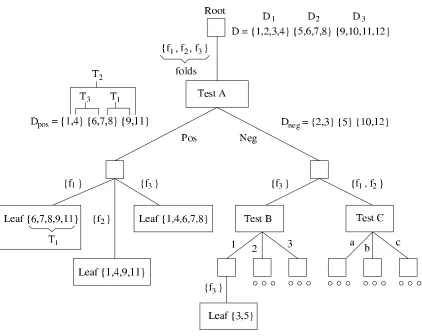
An example of a forest is shown in Figure 5. In this figure two kinds of internal nodes are represented. The small squares represent bifurcation points, points where the trees of different folds start to differ because different tests were selected. The larger rectangles represent tests that partition the relevant data set. The way in which the trees in the forest split the data sets is illustrated by means of an example data set of 12 elements on which a three-fold cross-validation is performed. Note that the memory consumption of a forest is (roughly) at most n+1 times that of a single tree (this happens when at the root different tests are obtained for all n folds plus the actual tree), which in practice is not problematic as long as n is relatively small. Cross-validation is often performed with
Figure 5: An example forest for a 3-fold cross-validation. At the root of the tree all folds select the same Test A. In the right subtree the different folds disagree on which test to select, so there is a bifurcation point: f3selects Test B whereas f1and f2select Test C.
When in the following we refer to nodes in the forest, we always refer to the test nodes, ignoring bifurcation points. For example, in Figure 5 the root node has five children, three of which are leaves.
3.2 Tree Induction Algorithms
We distinguish two types of algorithms for decision tree induction: depth first and level-wise algo-rithms.
3.2.1 DEPTHFIRSTTREE INDUCTION
The simplest way to adapt an ID3-like algorithm to perform cross-validation in parallel with the actual tree building, is to make it use the node refinement algorithm of Figure 4 and call the algorithm recursively for each child node created. Note that the number of such child nodes is now ∑f
i=1ri, with f the number of different tests selected as best test in some fold and ri the number of
possible results of the i-th test.
In this way, the above mentioned speedup is obtained as long as the same test is chosen in all cross-validations and in the actual tree. The more different tests are selected, the less speedup is achieved; and when in each fold a different test is selected, the speedup factor goes to 1 (all folds are handled separately).
To see how this process influences the total forest induction time, let us define tr(i)as the average
time that is needed to refine all the nodes of a single tree on level i for a data set of size|D|, and f(i)
as the average number of different tests selected on level i of the forest (averaged over all nodes on that level of the forest). The computational complexity of the whole forest building process for the parallel versions can then be approximated as
TOS,CV=tr(1) + f(1)tr(2) +f(2)tr(3) +···
Assuming that the refinement time is linear in the number of examples of a node that is to be refined,3we have for the serial version
TS=ntr(1) +ntr(2) +ntr(3) +···
(we obtain ntr(i)and not(n+1)tr(i)because the n folds have size n−n1|D|).
Thus the total speedup will be between 1 and n, and will be higher for stable problems (low
f(i)) than for unstable problems (most f(i)close to n+1).
3.2.2 LEVEL-WISE TREE INDUCTION
Most decision tree induction algorithms assume that all data reside in main memory. When inducing a tree from a large database, this may not be realistic: data have to be loaded from disk into main memory when needed, and then for efficiency reasons it is important to minimize the number of times each example needs to be loaded (thus minimizing disk access). To that aim alternative tree induction algorithms have been proposed (Mehta et al., 1996, Shafer et al., 1996) that build the tree one whole level at a time, where for each level one pass through the data is required. The idea is to go over the data and for each example, update the statistics for all possible tests in the node (of the currently lowest level of the tree) where the example belongs. For each node the best test is then selected from these statistics without more access to the data.
Since in these approaches, too, the computation of the quality of tests is split up into two phases (computing the statistics from the data, computing the test quality from the statistics), it is easy to see how such level-wise algorithms can be adapted. When processing one example, instead of looking up the single node in the tree where the example belongs, one should look up all the nodes in the forest where the example belongs (for an example not yet in a leaf this is at least one node and at most n−1 nodes, where n is the number of folds) and update the statistics in all these nodes. When data reside on the disk, the number of examples is typically large and also teis large (due
to external data access). The constant terms cithen become negligible very quickly, and the speedup
factor can approach n if a≥nte+tp
te+tu. Assuming that tpand tuare comparable, this will be true as soon as a≥n, which in practice often holds.
3.3 Space Complexity
The space requirements of the OS and CV algorithms differ from those of the serial algorithm in three major points: the statistics arrays are larger, we need to build a forest instead of one tree at a time, and there is a need to know for each example which data sets it is part of.
• The statistics arrays for OS and CV are indexed with Ti(and Di). This implies that their size
increases by a factor
O
(n) compared to algorithm S. In practice, this is acceptable because these arrays are small (e.g., two numbers for a binary classification problem, independent of the data set size). Depending on the implementation, CV may need more memory for statistics compared to OS because separate statistics are stored for Ti and Di and becausecertain intermediate sums must be stored.
• OS and CV store the cross-validation forest in memory. In the worst case, the size of this forest can increase up to
O
(n)times the size of a single decision tree. This happens if different tests are selected for all folds in the root node of the forest (so no sharing takes place). In practice this increase can be problematic for large trees and large n. For typical tree sizes andn=10, no problems would normally arise.
• Both OS and CV must know for each example to which training set it belongs (for instance, for the test e∈Ti in Fig. 3). We consider first the case of CV. Because Di are disjoint, one
can store the data in memory partitioned according to Di. This partition requires the same
amount of memory as is necessary for storing D when building the actual tree. This trick can not be used in the OS algorithm because we do not have the notion of Di. The OS algorithm
must store for each example to which sets it belongs. This can be done by adding n Booleans to each example, or n integers in the case of bagging (where a single example can occur multiple times in a given set). The total memory consumption increases with
O
(n×N), with a relatively small constant factor (size of a boolean or integer).Except for large n, we expect the extra memory needed by the parallel versions to be quite reasonable, and usually smaller than the memory that is taken by the data set itself (unless it has less than n attributes, in which the
O
(n×N)factor may dominate). This expectation remains to be validated empirically.3.4 Handling Numerical Attributes
The above description of the tree induction process still has an important shortcoming when com-pared to practical systems: it ignores the way in which numerical attributes are usually handled. This procedure is somewhat complicated, but due to its importance in practice we cannot avoid dis-cussing it here. We will see that this procedure, too, can be adapted for making an efficient parallel cross-validation possible.
A binary split of the form A≤v is typically used for numeric attributes. The first step in finding
split. Each of the different values of A is in general a useful split, though for classification tasks an optimization is possible: splits can only occur between class changes (Fayyad and Irani, 1993).
The algorithm uses total T S and left branch LS statistics. The total statistic is the class distribu-tion of the training examples in the node to be split. The left branch statistic is the class distribudistribu-tion of the examples for which the test A≤v succeeds. (The right branch statistic can be computed from
these as T S−LS.) Because the training examples are sorted it is possible to evaluate all useful splits
in one pass over the data. For each possible split, the left branch statistic LS is updated incremen-tally from the previous split, and the test’s quality is calculated based on T S and LS. For example, if some test A≤viyielded the distribution LS= [15,27](that is, out of 42 examples with A≤vi 15
are positive and 27 are negative), and the following three examples (sorted according to A) all have a positive class, then the next test to be evaluated is A≤vi+3and it has LS= [18,27].
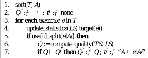
1. sort(T , A)
2. Q∗:=−∞; t∗:=none 3. for each example e in T
4. update statistics(LS, target(e))
5. if useful split(e[A]) then
6. Q := compute quality(T S, LS)
7. if Q>Q∗then Q∗:=Q ; t∗:=“A≤e[A]”
Figure 6: Finding the best split point for a numeric attribute.
The algorithm from Figure 6 can be adapted for parallel cross-validation as shown in Figure 7. The first step is again sorting the examples. Note that the time for finding a split is dominated by the sorting time as the number of examples increases. This is because sorting takes
O
(N log N). Algorithms designed to handle large data sets (e.g., SLIQ (Mehta et al., 1996), SPRINT (Shafer et al., 1996)) solve this problem by sorting numeric attributes only once before the actual induction starts. Algorithms like C4.5 (Quinlan, 1993a), that keep all the data in the main memory, do not use pre-sorting because this takes more memory (one needs at least an extra list with example indices for each numeric attribute) and because N is small. In both settings the sorting step will be more efficient for parallel cross-validation because we sort the original data set D and not the overlapping training sets Ti.After sorting, the algorithm iterates over the examples and evaluates useful splits for each fold. This can be implemented in two ways: either by updating the training set statistics (similar to the OS algorithm) or by updating the statistics on Di (similar to the CV algorithm). If the set of
useful splits for a numeric attribute is much smaller than the number of examples, then the second approach is better. This is the case for many (but not all) practical data sets because they either have many examples with identical values or because the class does not change often (e.g., if the class is correlated with the numeric attribute).
Algorithm 7 implements the version for finding the best split for a numeric attribute for each fold with statistics on Di. For each possible split, it first updates the left branch statistic for the
corresponding Di. After that it considers e[A]as possible split point for each fold j except for j=i
quality based on T S[Tj]and LS[Tj]. If the quality is better than the current best quality Q∗[Tj]then
the algorithm updates Q∗[Tj]and t∗[Tj]. When the algorithm finishes, t∗contains the best split for
each fold.
1. sort(D, A)
2. Q∗[T0...Tn]:=−∞; t∗[T0...Tn]:=none
3. for each example e in D
4. choose i such that e∈Di
5. update statistics(LS[Di], target(e))
6. for j :=0 to n
7. if i6= j and useful split(e[A], j) then
8. compute LS[Tj]from LS[Dk], k=1...n
9. Q := compute quality(T S[Tj], LS[Tj])
10. if Q>Q∗[Tj]then
11. Q∗[Tj]:=Q ; t∗[Tj]:=“A≤e[A]”
Figure 7: Finding the best splits for attribute Aifor all folds in parallel.
a
i
min max
v
1 v2 v3
test succeeds for all folds
test fails for all folds test succeeds for folds {3}
test succeeds for folds {2,3}
Figure 8: Different splits for a numeric attribute.
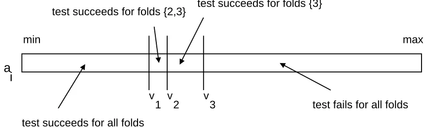
A problem with numeric attributes is that different folds are likely to select splits that appear different but are practically the same. Suppose for instance that two folds respectively select A< 42.3 and A<42.4 as optimal tests. These tests essentially indicate the same bound, even though the outcome of the computation is slightly different. Such slightly different splits still cause a bifurcation, and hence reduced sharing of computations. One would prefer a less strict test for equivalence of tests than just equality.
The solution we propose for this problem is as follows. Consider for example a 3-fold cross-validation as illustrated in Figure 8 (virtual fold 0 is not shown here). Fold 1 selects v1as split point,
fold 2 v2and fold 3 v3. The split points divide the range of A in three important intervals. The first
one is[min,v1], the second one(v1,v3]and the last one(v3,max]. Instead of creating a bifurcation
right sub-tree. Consider the examples in the left sub-tree. The test A≤vi succeeds for all folds i
and for all examples in S1= [min,v1]. The examples in S2= (v1,v3]are more difficult. Only some
of the tests succeed for these examples. But if the thresholds selected by different folds differ only slightly, S2 will be small. We mark each of the examples of S2 with the set of folds for which the corresponding test succeeds (see Figure 8). The examples in S1 can be split at lower levels of the forest by calculating statistics on Di. This is not possible anymore for the examples of S2. The
algorithm has to keep training set statistics for each fold for this type of examples and combine these when evaluating a test’s quality. The benefit of this extra book-keeping is that no bifurcation point is introduced in the forest when slightly different splits are selected for one numeric attribute.
3.5 Further Optimizations
As soon as different tests are selected for different folds, the forest induction process bifurcates in the sense that from that point onwards different trees in the forest will be handled independently. A further optimization that comes to mind, is removing redundancy among computations in these independently handled trees as well. Note that this is somewhat similar to what we just discussed concerning numerical attributes. The main difference is that up till now we handled “similar” tests, which differ only on few examples. The question we address here concerns tests that are entirely different.
Referring to Figure 5, among the different branches created by a bifurcation point (square node) there may still be some overlap with respect to the tests that will be considered in the child nodes, as well as the relevant examples. For instance, in the lower right of the forest in Figure 5, in the children of the “test B” node one needs to consider all tests except A and B, and in the children of the test C node one needs to consider all tests except A and C. Since the relevant example set for fold f3at that point ({2,3,5}) overlaps with that of folds f1and f2({2,3,5,10,12}), all tests besides A, B and C will give rise to some redundant computations.
As the amount of redundancy is lower here in this case than for very similar tests, we expect these optimizations to yield some, but not much, efficiency gain. Struyf and Blockeel (2001) have explored this idea in the context of an ILP (inductive logic programming) (Muggleton and De Raedt, 1994) system, and their results confirm this.
Finally, note that when a level-wise tree building method is adopted instead of a depth-first method, bifurcations automatically have a smaller effect in that data are still accessed only once. However, the statistics updates still need to be done multiple times. As mentioned before, this will yield a significant gain only if te>tu, which is typically not the case when the data reside in main
memory. Hence, the level-wise method does not seem to be a good optimization except in those cases where it would be considered anyway (data residing in external memory).
Here we will not discuss these optimizations any further but focus on the above described al-gorithm, which is simple and compatible with both tree induction approaches and can easily be integrated in existing tree induction systems.
4. Experimental Evaluation
• We distinguish three different algorithms, which we refer to as the unoptimized serial algo-rithm (S), the overlapping sets algoalgo-rithm (OS) which exploits overlap in different data sets, and the cross-validation algorithm (CV) which is tuned specifically for cross-validation and is the most optimized of these three.
• We look at both the ILP setting, which is characterized by a high te/tu and hence should
exhibit the highest efficiency gains, and the propositional setting, where gains are expected to be lower. Consequently, two different implementations will be used.
• The main sources of speedup that we can distinguish are
– removing redundancy in the evaluation of tests : present in the OS and CV algorithms; – removing redundancy in the updating of statistics: present only in the CV algorithm. – removing redundancy in the procedure for handling numerical attributes: in practice this
is an important component in the propositional setting (present in both OS and CV)
• We have mentioned that the OS algorithm is also usable for bagging, but the CV algorithm is not; hence we expect a smaller positive effect in the bagging context. We perform separate experiments to measure this.
• The proposed algorithms essentially trade time complexity for space complexity. Their scal-ing properties with respect to the latter are therefore of some concern. For this reason, mem-ory consumption of the algorithms will also be measured.
Based on this we structure the experimental section as follows. In the first subsection we in-troduce the used materials (implementations and data sets). In the second subsection we present timings for the cross-validation context. A breakdown of these timings into several components is presented and discussed; this gives more insight in the relative importance of the different opti-mizations. In the third subsection we present timing results for the bagging context, and in the last subsection we investigate the space complexity of the algorithms. In all cases we distinguish ILP and propositional results.
4.1 Materials
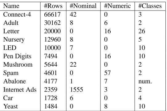
We have used the following data sets and implementations.
4.1.1 DATASETS
For our ILP experiments we have used the following data sets:
• SB (Simple Bongard) and CB (Complex Bongard): some artificially generated sets of the
so-called “Bongard” problems (De Raedt and Van Laer, 1995) (pictures are classified according to simple geometric patterns). SB contains 1453 examples with a simple underlying theory, CB 1521 examples with a more complex theory.
• Muta: the Mutagenesis data set (Srinivasan et al., 1996), an ILP benchmark (230 examples) • ASM: a subset of 999 examples of the so-called “Adaptive Systems Management” data set,
Name #Rows #Nominal #Numeric #Classes
Connect-4 66617 42 0 3
Adult 30162 8 6 2
Letter 20000 0 16 26
Nursery 12960 8 0 5
LED 10000 7 0 10
Pen Digits 7494 0 16 10
Mushroom 5644 22 0 2
Spam 4601 0 57 2
Abalone 4177 1 7 num.
Internet Ads 2359 1555 3 2
Car 1728 6 0 4
Yeast 1484 0 8 10
Table 1: The propositional data sets used.
• Mach: “Machines”, a tiny data set of 15 examples (Blockeel and De Raedt, 1998) that here
serves as a kind of limit case for situations where few examples are available.
For the propositional experiments we made a selection of the largest data sets available at the UCI Machine Learning Repository (Merz and Murphy, 1996). In Table 1 the data sets are listed in order of decreasing size. Most data sets are classification tasks except for “Abalone” where we try to predict the number of rings. The 1555 nominal attributes of “Internet Ads” form a sparse binary matrix.
4.1.2 IMPLEMENTATIONS
The systems we have used for these experiments consist of previously existing decision tree systems to which minimal modifications have been made to implement the algorithms described in this text. More specifically, for the ILP experiments we use the first order decision tree learner TILDE
(Blockeel and De Raedt, 1998) as implemented in the ACE-ILPROLOGdata mining tool (Blockeel
et al., 2002).4 Briefly, first order decision trees are decision trees where a test in a node is a first
order literal or conjunction, and a path from root to leaf can be interpreted as a Horn clause. Literals belonging to different nodes in such a path may share variables. The reader is referred to Blockeel and De Raedt (1998) for details.
For the experiments in the propositional setting we use the program CLUS, which in some sense is a specialized propositional version of TILDE capable of constructing classification, regression and clustering trees (Blockeel et al., 1998). CLUSis implemented in Java and is available from the
authors upon request.
In both cases the changes to the original system consisted of implementing the algorithms in Figures 3 and 4 as well as the “forest” data structure and the corresponding induction procedure. In addition the optimized procedure for handling numerical attributes was added to CLUS. (TILDE
does not have a special procedure for numerical attributes, for reasons not relevant here.) Except for these points, the different versions of TILDE/ CLUSuse exactly the same implementation.
4.1.3 SETTINGS
All programs were run with default settings except for the following. We set the stopping criterion of CLUSso that no leaves smaller than 10 examples can be generated. This is a reasonable value given the data set sizes. TILDE, like other ILP systems, employs a declarative language bias formalism
to specify which tests can occur in nodes. The details of this formalism are out of the scope of this article, but we mention that with the employed language specification, the number of tests evaluated in each node (the a parameter) varied from 3 to a few hundred (as tests are first-order clauses, their number may vary greatly even among nodes of the same tree).
4.2 Breakdown of Computational Cost
In a first series of experiments, we try to gain insight in the speedups that the proposed algorithms may yield in a number of specific practical cases. Our main question is: how much more efficiently can cross-validation be performed by using the proposed algorithms? From this question several more detailed questions arise, such as how speedups in the ILP setting compare to those in the propositional setting, what the contributions of the different optimizations are, and how the speedups vary with the number of examples and number of folds.
4.2.1 RESULTS FOR THEILP SETTING
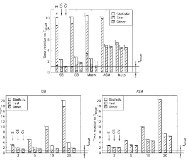
Figure 9 plots cross-validation timing results for tenfold cross-validation for all data sets, as well as for n-fold cross-validation with varying n for two selected data sets. The three consecutive bars always represent TS, TOSand TCV (the times needed for cross-validation plus induction of the actual
tree), relative to Tactual (the time needed for induction of the actual tree). Each bar indicates the
average run time of 10 different runs; 90% confidence intervals for this average are plotted.
The bars are broken down into components indicating the proportion of time spent on statistics updates, running tests on the data set to determine the best test, and “other”, that is, all other com-putations (including the partitioning step).5 The proposed optimizations mostly influence the first two components. More specifically, for the OS algorithm the test time is strongly reduced, while the CV algorithm adds to this a strong reduction in statistics update time.
In general the graphs in Figure 9 confirm our expectations. Comparing the total time to Tactual,
the lowest overhead is achieved for Simple Bongard, which has a relatively large number of exam-ples and a simple theory. The simplicity of the true theory causes the induced trees to be exactly the same in most folds, yielding little bifurcation. For Complex Bongard, the effect of bifurcation is more prominent. For ASM, a real-world data set for which a perfect theory may not exist, the overhead of cross-validation is relatively high (but still better than that for the serial algorithm). For Machines, the overhead is relatively large but still smaller than for the serial algorithm. This shows that even for very small example sets the parallel algorithm yields a speedup.
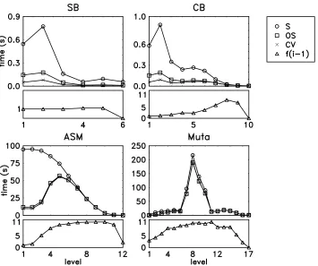
For Mutagenesis we obtained less good results. Two factors turned out to be responsible for this: instability of the trees, and high variance in the complexity of testing examples. The latter is due to the fact that first-order queries have exponential worst-case complexity; most of them are reasonably fast, but very few of them may time-wise dominate the others. Such behaviour typically occurs at lower levels of the tree, as will be confirmed when we look at Figure 10.
Figure 9: Timings for cross-validation experiments in an ILP setting; upper graph: for all data sets, with n=10; lower graphs: for selected data sets with n varying from 3 to 20.
The lower part of Figure 9 shows how cross-validation overhead varies with the number of folds for the CB and ASM data sets. The result for CB confirms our expectation that n has a small influence on the total time, but for ASM the overhead increases with increasing n.
The latter result can be understood by looking at the graphs in Figure 10, where the total time spent on each level of the tree by the parallel and the serial procedure is plotted, together with the
Figure 10: For four different data sets, the graphs show the total refinement time spent at each level
i of the forest by the different algorithms (upper part of each graph) and the number of
Figure 11: Timings for cross-validation experiments in a propositional setting, for all data sets, with
n=10.
4.2.2 RESULTS FOR THEPROPOSITIONAL SETTING
Results for the propositional setting are shown in Figure 11. The same breakdown into components has been made as in the previous figures, but now an extra component has been singled out: the time consumed by the numerical attribute handling procedure. Due to the sorting process that it entails, this procedure consumes a reasonably large proportion of the total induction time and consequently optimizations in this procedure have a large effect on the total runtimes.
In general these timings show the same tendencies as for the ILP setting, with the following notable differences:
• The different components are more balanced than in the ILP case: the proportion of time
dedicated to running tests on examples tends to be lower, while the proportion dedicated to statistics updates is higher.
• Optimizing the numerical attribute handling procedure turns out to play an important role. For data sets with many numerical attributes a significant speedup is obtained in this way.
• The time for the statistics updates tends to slightly increase with the OS optimization. This is due to the fact that more administrative work is needed (e.g., more lookups are necessary to find the correct counter to be incremented). This effect is not unexpected; in the ILP setting it was less obvious because of the proportionally smaller time that statistics updates take.
• In a few cases (most notably Abalone) the statistics update time increases for the CV opti-mization. The reason for this is the procedure for handling numerical attributes. As men-tioned in Section 3.4, when the number of splits considered for a single numerical attribute is in the same order of magnitude as the number of examples, this causes a significant overhead compared to updating Tidirectly.6
Figure 12: 90% confidence intervals (one per data set) for the mean speedup obtained during n-fold cross-validation for varying n.
• For the Car data set, OS yields an efficiency loss. To interpret this, we have to mention that the induction process for this data set finished very quickly. One problem is that this makes accurate timing more difficult. Careful checking revealed however that the increase of the total runtime as shown on the graph is accurate: the OS optimization causes a small increase in runtime and this is due to the increased statistics update time. In absolute terms the increase is very small, but compared to the small total time it represents a clear overhead.
Our overall conclusions from this are that all optimizations together definitely have a positive effect (this was so in all data sets we used), but the individual impact of a single optimization varies:
• For data sets with many numerical attributes, the optimization for handling numerical at-tributes plays an important role, while the CV optimization has a limited or even negative effect.
• For data sets without numerical attributes, the CV optimization yields a significant extra gain over the OS version.
Figures 12 and 13 give an idea of how the measured speedups depend on parameters such as the number of examples and the number of folds. Consistent with expectations, there is a clear increase in the speedup factor with increasing number of folds, and a small increase with the data set size.
In an attempt to identify any further influences on the speedup factor, we have grown a small meta decision tree7with as target a 2-D vector containing the measured speedup for the CV and OS algorithms. This tree is shown in Figure 14. Note that the generalisability of the precise speedup predictions is not evaluated here. We are mainly interested in interpreting the tests in the tree. The influences revealed by the tree can be generalized with high confidence, in the sense that we can explain them using our knowledge of the problem and implementation.
The tree confirms that the existence of numerical attributes and the number of examples play a role, and identifies in addition the following influences:
Figure 13: 90% confidence intervals (one per data set) for the mean speedup obtained during 10-fold cross-validation for varying sample sizes (indicated as percentage of the original data set).
• tree size (number of nodes in the tree): smaller trees are usually more stable, and the number
of examples considered in each node is on average relatively large in this case, so we can expect higher gain for smaller trees.
• number of classes : if a dataset has more classes then the statistics arrays are larger and the
proportional time for computing the Tistatistics from the Diand for computing the heuristics
becomes greater. This part is not affected by the optimizations. Therefore having more classes causes the speedup ratio to decrease.
• existence of numerical attributes : the tree confirms that the existence of numerical attributes
increases the speedup obtainable with OS but decreases that with CV.
Finally, the tree suggests that the CV optimization yields the largest gain over the OS optimization (6.30 versus 2.06) in the case of large data sets and small trees, that is, where the theoretically derived upper bounds (influenced by n, a and for OS also te/tu) on the speedups are most easily
achieved.
4.3 Usefulness of These Algorithms for Bagging
As mentioned, the OS algorithms can also be used in a bagging context but the CV version cannot. Our theoretical analysis suggests that the OS algorithm may still yield substantial speedups for the ILP case but less so for the propositional case.
Figures 15 and 16 present results of experiments where the OS algorithm in TILDEand CLUSis
run on n sets, each constructed by randomly drawing with replacement N elements from a data set of N elements, exactly as is normally done for bagging. The figures show the timings for bagging experiments with n=25 for all data sets, and for varying n on a number of selected data sets.
Rows > 4,601
+--yes: TreeSize > 48
| +--yes: Numeric > 0
| | +--yes: [2.57, 2.74]
| | +--no: [1.90, 4.09]
| +--no: [2.06, 6.30]
+--no: Classes > 2
+--yes: [1.31, 1.51]
+--no: [1.64, 2.00]
Figure 14: Meta decision tree that predicts the speedup; the first number is the predicted speedup for the OS version, the second for the CV version.
evaluation is offset by the more complex statistics updates. In those cases where a relatively high gain (say, a factor 2 speedup) is obtained, it turns out this can largely be attributed to the optimized procedure for handling numerical attributes.
Figure 17 shows how the speedup evolves with the number of bags and the sample size. The dependency of the speedup on the number of sets is smaller than for cross-validation because in contrast to the latter, the sets do not become more similar when there are more of them. There is again a small positive effect of sample size, indicating that for larger data sets the probability of the OS optimization actually slowing down the systems becomes small. Nevertheless, speedups are limited to a factor of about 3.
4.4 Space Complexity
The space complexity issue, from a practical point of view, boils down to the following: how much extra memory will a decision tree learning system need if it employs the OS or CV algorithms instead of the serial one?
For both TILDE and CLUS, the memory consumption of the process (as reported by the Unix
toolps) was measured at three points in time: after loading the system, after loading the data, and after running an n-fold cross-validation. Like previously, this was done for all data sets for n=10, and for selected data sets with varying n.
Results of these measurements are shown in Figures 18 and 19. In the ILP setting, memory con-sumption turns out to be relatively independent of the number of folds. This is because the memory allocated for loading the system and the data and for running the queries outweighs the memory consumption of the trees themselves. The total memory consumption monotonically increases with the number of folds, but at such a low rate that performing for instance a 20-fold cross-validation with one of the parallel algorithms barely increases memory consumption, compared to the serial version.
Figure 15: Timings for Bagging experiments in an ILP setting; upper graph: for all data sets, with
n=25; lower graphs: for selected data sets with n varying from 10 to 100.
Figure 17: Timings for Bagging experiments in a propositional setting, 90% confidence intervals shown for the mean speedup for all datasets; left: with n=10, 25, 50, 100, right: with n = 25 and different samples sizes.
increasing n quickly becomes problematic for this data set, but has a very small effect for the other data sets.
4.5 A Summary of the Experimental Results
Summarising our findings in this experimental section, we list the following conclusions:
• Both in the propositional and the ILP setting, the proposed optimizations almost always yield efficiency gains.
• The efficiency gains are highest for cross-validation. For bagging smaller efficiency gains are to be expected.
• We identified two factors that are detrimental to the efficiency gain: high variance of test complexity (which occurs typically in the ILP setting, not in the propositional setting) and instability of the problem (different folds yielding very different trees). Note that since bag-ging is most useful for unstable problems, the latter factor imposes a further limitation on the usefulness of the techniques for bagging.
• For data sets with many numerical attributes, the CV optimization may yield little or no gain over the OS optimization, while the optimization related to numerical attribute handling has a large effect.
• The memory usage of the parallel algorithms is in general not problematic. We have encoun-tered one case where it would become so if n becomes large.
Figure 18: Memory consumption of the ILP system ACE during cross-validation of TILDE; upper graph: all data sets using 10 folds; lower graphs: selected data sets using a varying number of folds.
Figure 20: Memory consumption of CLUSduring cross-validation as a function of folds.
5. Applicability of the Techniques
Although we have studied efficient cross-validation in the context of decision trees, the principles explained here are also applicable outside this domain. For instance, rule set induction systems (e.g., Quinlan, 1993b, Clark and Niblett, 1989) typically build a rule by consecutively adding a “best” condition to it until no further improvement occurs. Similar to our forest-building algorithm, cross-validation of such rules could be performed in parallel with the construction of the actual rule set, avoiding redundant computations.
It is less clear, however, how the technique could be used with models that contain only continu-ous parameters, such as neural networks. We obtain the greatest speedups for stable trees, where the same test is chosen in different folds. With continuous models, no computations will ever be exactly the same, hence removal of exactly redundant computations as explained here will in general not be possible.
It should be pointed out that the proposed techniques concern the tree building phase only. This phase is typically followed by tree post-pruning, and may be preceded by data pre-processing, such as discretization of attributes (Fayyad and Irani, 1993). While these other phases usually take much less time than the tree building phase, when they are not negligible and n is large they may become the bottleneck, limiting the usefulness of our approach (unless optimizations similar to the ones discussed here are also possible in these phases).
6. Conclusions
We have shown that in the context of decision tree induction the benefits of cross-validation are available for a relatively low overhead, if the cross-validation is carefully integrated with the normal tree building process. The overhead is smallest if data access is slow (complex tests, or data residing on disk), but even for the case that is hardest to improve (propositional data in main memory) a clear efficiency gain compared to straightforward implementations of cross-validation can be obtained.
cases it was still smaller than for the serial cross-validation procedure, and in the best cases there was only a small overhead over the normal tree induction process. Further experiments have shown that in practice, significant speedups can be obtained even for relatively small data sets (a few thou-sand examples), and that the speedups become larger when smaller trees are learnt (which typically indicates better stability).
In the context of bagging, a similar technique can be used, although here it can be less optimized than for cross-validation. Experimental results indicate that typically only relatively small gains are obtained in this case. The main exception to this is when the data contains many numerical attributes: in that case having a single sorting pass over the full training data set is advantageous.
A number of guidelines have been distilled from this work. They can be summarized as follows: implementing the proposed techniques is most worthwhile for ILP systems; it may be worthwhile for propositional systems if one expects frequent use of cross-validation; it is probably less worth-while for bagging alone, but can fruitfully be exploited in that context if it is available anyway.
The ideas underlying our approach are also applicable outside the decision tree context, e.g., for rule induction, but not immediately for induction of models that have only continuous parameters.
Related work includes that of Moore and Lee (1994), who discuss efficient cross-validation in the context of model selection. Their approach differs substantially from ours in that they obtain efficiency by quickly abandoning models that have a low probability of ever becoming the best model after a few examples have been seen. That is, they save on the number of cases a model is evaluated on during cross-validation, whereas our work focuses on removing redundancy in the model building process itself.
Kohavi (1995) and Utgoff (1997) note that incremental learning systems have the advantage that leave-one-out cross-validation can be performed efficiently by learning once using the whole data set and then “decrementally” adapting the theory, each time leaving one example out from the data set. In the case of Utgoff’s incremental decision tree learner, the computations involved in this seem quite similar to the ones performed by our procedure. However, no experimental results are reported by Utgoff (the cross-validation procedure is not the main topic of that article).
Blockeel et al. (2002) discuss a technique similar to the one described here. The main difference is in the kind of redundancies that are removed; here the redundancies arise from running the same test in different folds of a cross-validation, whereas Blockeel et al. (2002) consider redundancies caused by similarities in different tests (the tests being first-order conjunctions, which might be similar up to one literal). Both approaches can easily be combined, as shown by Struyf and Blockeel (2001).
Acknowledgements
The authors are respectively a post-doctoral fellow and research assistant of the Fund for Scien-tific Research of Flanders (Belgium). They wish to thank Ron Kohavi for providing very useful pointers and comments on this work, as well as an ICML-2001 attendant who pointed out the pos-sible usefulness of this technique for bagging. They also thank the anonymous reviewers for their extensive comments on a previous version of this text. The authors gratefully acknowledge Perot Systems Nederland / Syllogic for providing the ASM data. The cooperation between Perot Systems Nederland and the authors was supported by the European Union’s Esprit Project 28623 (Aladin).
References
H. Blockeel and L. De Raedt. Top-down induction of first order logical decision trees. Artificial
Intelligence, 101(1-2):285–297, 1998.
H. Blockeel, L. De Raedt, and J. Ramon. Top-down induction of clustering trees. In Proceedings of
the Fifteenth International Conference on Machine Learning, pages 55–63. Morgan Kaufmann,
San Francisco, California, 1998.
H. Blockeel, L. Dehaspe, B. Demoen, G. Janssens, J. Ramon, and H. Vandecasteele. Improving the efficiency of inductive logic programming through the use of query packs. Journal of Artificial
Intelligence Research, 16:135–166, 2002.
L. Breiman. Bagging predictors. Machine Learning, 24(2):123–140, 1996.
L. Breiman, J.H. Friedman, R.A. Olshen, and C.J. Stone. Classification and Regression Trees. Wadsworth, Belmont, 1984.
P. Clark and T. Niblett. The CN2 algorithm. Machine Learning, 3(4):261–284, 1989.
L. De Raedt and W. Van Laer. Inductive constraint logic. In Proceedings of the Sixth International
Workshop on Algorithmic Learning Theory, volume 997 of Lecture Notes in Artificial Intelli-gence, pages 80–94. Springer-Verlag, Berlin, 1995.
U.M. Fayyad and K.B. Irani. Multi-interval discretization of continuous-valued attributes for clas-sification learning. In Proceedings of the Thirteenth International Joint Conference on Artificial
Intelligence, pages 1022–1027. Morgan Kaufmann, San Francisco, California, 1993.
Y. Freund and R. E. Schapire. Experiments with a new boosting algorithm. In Proceedings of the
Thirteenth International Conference on Machine Learning, pages 148–156. Morgan Kaufmann,
San Francisco, California, 1996.
R. Kohavi. The power of decision tables. In Proceedings of the 8th European Conference on
Ma-chine Learning, volume 912 of Lecture Notes in Artificial Intelligence, pages 174–189.
Springer-Verlag, Berlin, 1995.
R. Kohavi and G. John. Automatic parameter selection by minimizing estimated error. In
Ma-chine Learning: Proceedings of the Twelfth International Conference, pages 304–312. Morgan
Kaufmann, San Francisco, California, 1995.
M. Mehta, R. Agrawal, and J. Rissanen. SLIQ: A fast scalable classifier for data mining. In
Proceedings of the Fifth International Conference on Extending Database Technology, volume
1057 of Lecture Notes in Computer Science, pages 18–32. Springer-Verlag, Berlin, 1996.
C.J. Merz and P.M. Murphy. UCI repository of machine learning databases
[http://www.ics.uci.edu/˜mlearn/mlrepository.html]. Department of Information and
Computer Science, University of California, Irvine, California, 1996.
A.W. Moore and M.S. Lee. Efficient algorithms for minimizing cross validation error. In
Pro-ceedings of the 11th International Conference on Machine Learning, pages 190–198. Morgan
Kaufmann, San Francisco, California, 1994.
S. Muggleton and L. De Raedt. Inductive logic programming : Theory and methods. Journal of
Logic Programming, 19,20:629–679, 1994.
J. R. Quinlan. Induction of decision trees. Machine Learning, 1:81–106, 1986.
J. R. Quinlan. C4.5: Programs for Machine Learning. Morgan Kaufmann series in machine learn-ing. Morgan Kaufmann, San Francisco, California, 1993a.
J.R. Quinlan. FOIL: A midterm report. In Proceedings of the 6th European Conference on Machine
Learning, volume 667 of Lecture Notes in Artificial Intelligence, pages 3–20. Springer-Verlag,
Berlin, 1993b.
J.C. Shafer, R. Agrawal, and M. Mehta. SPRINT: A scalable parallel classifier for data mining. In Proceedings of the 22th International Conference on Very Large Databases, pages 544–555. Morgan Kaufmann, San Francisco, California, 1996.
A. Srinivasan, S.H. Muggleton, M.J.E. Sternberg, and R.D. King. Theories for mutagenicity: A study in first-order and feature-based induction. Artificial Intelligence, 85(1,2): 277–299, 1996.
J. Struyf and H. Blockeel. Efficient cross-validation in ILP. In Proceedings of the Eleventh
Interna-tional Conference on Inductive Logic Programming, volume 2157 of Lecture Notes in Artificial Intelligence, pages 228–239. Springer-Verlag, Berlin, 2001.
L. Todorovski and S. Dˇzeroski. Combining multiple models with meta decision trees. In
Pro-ceedings of the Fourth European Conference on Principles and Practice of Data Mining and Knowledge Discovery (PKDD-2000), volume 1910 of Lecture Notes in Artificial Intelligence,
pages 54–64. Springer-Verlag, Berlin, 2000.