Efficient Active Learning of Halfspaces: An Aggressive Approach

Efficient Active Learning of Halfspaces: An Aggressive Approach

Alon Gonen ALONGNN@CS.HUJI.AC.IL

The Rachel and Selim Benin School of Computer Science and Engineering The Hebrew University

Givat Ram, Jerusalem 91904, Israel

Sivan Sabato SIVAN.SABATO@MICROSOFT.COM

Microsoft Research New England 1 Memorial Drive

Cambridge, MA, 02142

Shai Shalev-Shwartz SHAIS@CS.HUJI.AC.IL

The Rachel and Selim Benin School of Computer Science and Engineering The Hebrew University

Givat Ram, Jerusalem 91904, Israel

Editor:John Shawe-Taylor

Abstract

We study pool-based active learning of half-spaces. We revisit the aggressive approach for active learning in the realizable case, and show that it can be made efficient and practical, while also having theoretical guarantees under reasonable assumptions. We further show, both theoretically and experimentally, that it can be preferable to mellow approaches. Our efficient aggressive active learner of half-spaces has formal approximation guarantees that hold when the pool is separable with a margin. While our analysis is focused on the realizable setting, we show that a simple heuristic allows using the same algorithm successfully for pools with low error as well. We further compare the aggressive approach to the mellow approach, and prove that there are cases in which the aggressive approach results in significantly better label complexity compared to the mellow approach. We demonstrate experimentally that substantial improvements in label complexity can be achieved using the aggressive approach, for both realizable and low-error settings.

Keywords: active learning, linear classifiers, margin, adaptive sub-modularity

1. Introduction

We consider pool-based active learning (McCallum and Nigam, 1998), in which a learner receives a pool of unlabeled examples, and can iteratively query a teacher for the labels of examples from the pool. The goal of the learner is to return a low-error prediction rule for the labels of the examples, using a small number of queries. The number of queries used by the learner is termed itslabel complexity. This setting is most useful when unlabeled data is abundant but labeling is expensive, a common case in many data-laden applications. A pool-based algorithm can be used to learn a classifier in the standard PAC model, while querying fewer labels. This can be done by first drawing a random unlabeled sample to be used as the pool, then using pool-based active learning to identify its labels with few queries, and then using the resulting labeled sample as input to a regular “passive” PAC-learner.

Most active learning approaches can be loosely described as more ‘aggressive’ or more ‘mellow’. A more aggressive approach is one in which only highly informative queries are requested (where the meaning of ‘highly informative’ depends on the particular algorithm) (Tong and Koller, 2002; Balcan et al., 2007; Dasgupta et al., 2005), while the mellow approach, first proposed in the CAL algorithm (Cohn et al., 1994), is one in which the learner essentially queries all the labels it has not inferred yet.

approach can guarantee an exponential improvement in label complexity, compared to passive learning (Bal-can et al., 2006a). This exponential improvement depends on the properties of the distribution, as quantified by theDisagreement Coefficient proposed in Hanneke (2007). Specifically, when learning half-spaces in Euclidean space, the disagreement coefficient implies a low label complexity when the data distribution is uniform or close to uniform. Guarantees have also been shown for the case where the data distribution is a finite mixture of Gaussians (El-Yaniv and Wiener, 2012).

An advantage of the mellow approach is its ability to obtain label complexity improvements in the agnos-tic setting, which allows an arbitrary and large labeling error (Balcan et al., 2006a; Dasgupta et al., 2007). Nonetheless, in the realizable case the mellow approach is not always optimal, even for the uniform dis-tribution (Balcan et al., 2007). In this work we revisit the aggressive approach for the realizable case, and in particular for active learning of half-spaces in Euclidean space. We show that it can be made efficient and practical, while also having theoretical guarantees under reasonable assumptions. We further show, both theoretically and experimentally, that it can sometimes be preferable to mellow approaches.

In the first part of this work we construct an efficient aggressive active learner for half-spaces in Euclidean space, which is approximately optimal, that is, achieves near-optimal label complexity, if the pool is separable with a margin. While our analysis is focused on the realizable setting, we show that a simple heuristic allows using the same algorithm successfully for pools with low error as well. Our algorithm for halfspaces is based on a greedy query selection approach as proposed in Tong and Koller (2002) and Dasgupta (2005). We obtain improved target-dependent approximation guarantees for greedy selection in a general active learning setting. These guarantees allow us to prove meaningful approximation guarantees for halfspaces based on a margin assumption.

In the second part of this work we compare the greedy approach to the mellow approach. We prove that there are cases in which this highly aggressive greedy approach results in significantly better label complexity compared to the mellow approach. We further demonstrate experimentally that substantial improvements in label complexity can be achieved compared to mellow approaches, for both realizable and low-error settings. The first greedy query selection algorithm for learning halfspaces in Euclidean space was proposed by Tong and Koller (2002). The greedy algorithm is based on the notion of a version space: the set of all hypotheses in the hypothesis class that are consistent with the labels currently known to the learner. In the case of halfspaces, each version space is a convex body in Euclidean space. Each possible query thus splits the current version space into two parts: the version space that would result if the query received a positive label, and the one resulting from a negative label. Tong and Koller proposed to query the example from the pool that splits the version space as evenly as possible. To implement this policy, one would need to calculate the volume of a convex body in Euclidean space, a problem which is known to be computationally intractable (Brightwell and Winkler, 1991). Tong and Koller thus implemented several heuristics that attempt to follow their proposed selection principle using an efficient algorithm. For instance, they suggest to choose the example which is closest to the max-margin solution of the data labeled so far. However, none of their heuristics provably follow this greedy selection policy.

The label complexity of greedy pool-based active learning algorithms can be analyzed by comparing it to the best possible label complexity of any pool-based active learner on the same pool. Theworst-case label complexityof an active learner is the maximal number of queries it would make on the given pool, where the maximum is over all the possible classification rules that can be consistent with the pool according to the given hypothesis class. Theaverage-case label complexityof an active learner is the average number of queries it would make on the given pool, where the average is taken with respect to some fixed probability distributionPover the possible classifiers in the hypothesis class. For each of these definitions, the optimal label complexity is the lowest label complexity that can be achieved by an active learner on the given pool. Since implementing the optimal label complexity is usually computationally intractable, an alternative is to implement an efficient algorithm, and to guarantee a bounded factor of approximation on its label complexity, compared to the optimal label complexity.

O(log(1/pmin)), wherepminis the minimal probability of any possible labeling of the pool, if the classifier is

drawn according to the fixed distribution. Golovin and Krause (2010) extended Dasgupta’s result and showed that a similar bound holds for an approximate greedy rule. They also showed that the approximation factor for the worst-case label complexity of an approximate greedy rule is also bounded byO(log(1/pmin)), thus

extending a result of Arkin et al. (1993). Note that in the worst-case analysis, the fixed distribution is only an analysis tool, and does not represent any assumption on the true probability of the possible labelings.

Returning to greedy selection of halfspaces in Euclidean space, we can see that the fixed distribution over hypotheses that matches the volume-splitting strategy is the distribution that draws a halfspace uniformly from the unit ball.1The analysis presented above thus can result in poor approximation factors, since if there are instances in the pool that are very close to each other, thenpminmight be very small.

We first show that mild conditions suffice to guarantee that pmin is bounded from below. By proving a

variant of a result due to Muroga et al. (1961), we show that if the examples in the pool are stored using number of a finite accuracy 1/c, thenpmin≥(c/d)d

2

, whered is the dimensionality of the space. It follows that the approximation factor for the worst-case label complexity of our algorithm is at mostO(d2_log(d/c)).

While this result provides us with a uniform lower bound on pmin, in many real-world situations the

probability of the target hypothesis (i.e., one that is consistent with the true labeling) could be much larger thanpmin. A noteworthy example is when the target hypothesis separates the pool with a margin ofγ. In this

case, it can be shown that the probability of the target hypothesis is at leastγd_{, which can be significantly}

larger than pmin. An immediate question is therefore: can we obtain atarget-dependent label complexity

approximation factor that would depend on the probability of the target hypothesis, P(h), instead of the minimal probability of any labeling?

We prove that such a target dependent bounddoes nothold for a general approximate-greedy algorithm. To overcome this, we introduce an algorithmic change to the approximate greedy policy, which allows us to obtain a label complexity approximation factor of log(1/P(h)). This can be achieved by running the approximate-greedy procedure, but stopping the procedure early, before reaching a pure version space that exactly matches the labeling of the pool. Then, an approximate majority vote over the version space, that is, a random rule which approximates the majority vote with high probability, can be used to determine the labels of the pool. This result is general and holds for any hypothesis class and distribution. For halfspaces, it implies an approximation-factor guarantee ofO(dlog(1/γ)).

We use this result to provide an efficient approximately-optimal active learner for half-spaces, called

ALuMA, which relies on randomized approximation of the volume of the version space (Kannan et al., 1997). This allows us to prove a margin-dependent approximation factor guarantee for ALuMA. We further show an additional, more practical implementation of the algorithm, which has similar guarantees under mild conditions which often hold in practice. The assumption of separation with a margin can be relaxed if a lower bound on the total hinge-loss of the best separator for the pool can be assumed. We show that under such an assumption a simple transformation on the data allows running ALuMA as if the data was separable with a margin. This results in approximately optimal label complexity with respect to the new representation.

We also derive lower bounds, showing that the dependence of our label-complexity guarantee on the accuracyc, or the margin parameter γ, is indeed necessary and is not an artifact of our analysis. We do not know if the dependence of our bounds ond is tight. It should be noted that some of the most popular learning algorithms (e.g., SVM, Perceptron, and AdaBoost) rely on a large-margin assumption to derive dimension-independent sample complexity guarantees. In contrast, here we use the margin for computational reasons. Our approximation guarantee depends logarithmically on the margin parameter, while the sample complexities of SVM, Perceptron, and AdaBoost depend polynomially on the margin. Hence, we require a much smaller margin than these algorithms do. In a related work, Balcan et al. (2007) proposed an active learning algorithm with dimension-independent guarantees under a margin assumption. These guarantees hold for a restricted class of data distributions.

In the second part of this work, we compare the greedy approach to the mellow approach of CAL in the realizable case, both theoretically and experimentally. Our theoretical results show the following:

1. In the simple learning setting of thresholds on the line, our margin-based approach is preferable to the mellow approach when the true margin of the target hypothesis is large.

2. There exists a distribution in Euclidean space such that the mellow approach cannot achieve a signifi-cant improvement in label complexity over passive learning for halfspaces, while the greedy approach achieves such an improvement using more unlabeled examples.

3. There exists a pool in Euclidean space such that the mellow approach requires exponentially more labels than the greedy approach.

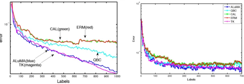
We further compare the two approaches experimentally, both on separable data and on data with small er-ror. The empirical evaluation indicates that our algorithm, which can be implemented in practice, achieves state-of-the-art results. It further suggests that aggressive approaches can be significantly better than mellow approaches in some practical settings.

2. On the Challenges in Active Learning for Halfspaces

The approach we employ for active learning does not provide absolute guarantees for the label complexity of learning, but a relative guarantee instead, in comparison with the optimal label complexity. One might hope that an absolute guarantee could be achieved using a different algorithm, for instance in the case of half-spaces. However, the following example from Dasgupta (2005) indicates that no meaningful guarantee can be provided that holds for all possible pools.

Example 1 Consider a distribution inRd_{for any d≥3. Suppose that the support of the distribution is a set of} evenly-distributed points on a two-dimensional sphere that does not circumscribe the origin, as illustrated in the following figure. As can be seen, each point can be separated from the rest of the points with a halfspace.

In this example, to distinguish between the case in which all points have a negative label and the case in which one of the points has a positive label while the rest have a negative label, any active learning algorithm will have to query every point at least once. It follows that for anyε>0, if the number of points is 1/ε, then the label complexity to achieve an error of at mostεis 1/ε. On the other hand, the sample complexity of passive learning in this case is order of 1_εlog1_ε, hence no active learner can be significantly better than a passive learner on this distribution.

Since we provide margin-dependent guarantees, one may wonder if a margin assumption alone can guar-antee that few queries suffice to learn the half-space. This is not the case, as evident by the following variation of Example 1.

Example 2 Letγ∈(0,1₂)be a margin parameter. Consider a pool of m points inRd, such that all the points are on the unit sphere, and for each pair of points x1and x2,hx1,x2i ≤1−2γ. It was shown in Shannon (1959) that for any m_≤O(1/γd_{), there exists a set of points that satisfy the conditions above. For any point} x in such a pool, there exists a (biased) halfspace that separates x from the rest of the points with a margin ofγ. This can be seen by letting w=x and b=1−γ. Then_hw,x_{i −}b=γwhile for any z₆=x in the set,

These examples show that there are “difficult” pools, where no active learner can do well. The advantage of the greedy approach is that the optimal label complexity is used as a natural measure of the difficulty of the pool.

At first glance it might seem that there are simpler ways to implement an efficient greedy strategy for halfspaces, by using a different distribution over the hypotheses. For instance, if there aremexamples in

d dimensions, Sauer’s lemma states that the effective size of the hypothesis class of halfspaces will be at mostmd. One can thus use the uniform distribution over this finite class, and greedily reduce the number of possible hypotheses in the version space, obtaining adlog(m)factor relative to the optimal label complexity. However, a direct implementation of this method will be exponential ind, and it is not clear whether this approach has a polynomial implementation.

Another approach is to discretize the version space, by considering only halfspaces that can be represented as vectors on ad-dimensional grid{−1,−1+c, . . . ,1−c,1}d_{. This results in a finite hypothesis class of size} (2/c+1)d, and we get an approximation factor ofO(dlog(1/c))for the greedy algorithm, compared to an optimal algorithm on the same finite class. However, it is unknown whether a greedy algorithm for reducing the number of such vectors in a version space can be implemented efficiently, since even determining whether a single grid point exists in a given version space is NP-hard (see, e.g., Matouˇsek, 2002, Section 2.2). In particular, the volume of the version space cannot be used to estimate this quantity, since the volume of a body and the number of grid points in this body are not correlated. For example, consider a line inR2, whose volume is 0. It can contain zero grid points or many grid points, depending on its alignment with respect to the grid. Therefore, the discretization approach is not straightforward as one might first assume. In fact, if this approach is at all computationally feasible, it would probably require the use of some approximation scheme, similarly to the volume-estimation approach that we describe below.

Yet another possible direction for pool-based active learning is to greedily select a query whose answer would determine the labels of the largest amount of pool examples. The main challenge in this direction is how to analyze the label complexity of such an algorithm: it is unclear whether competitiveness with the optimal label complexity can be guaranteed in this case. Investigating this idea, both theoretically and experimentally, is an important topic for future work. Note that the CAL algorithm (Cohn et al., 1994), which we discuss in Section 6, can be seen as implementing a mellow version of this approach, since it decreases the so-called “disagreement region” in each iteration.

3. Definitions and Preliminaries

In pool-based active learning, the learner receives as input a set of instances, denotedX={x1, . . . ,xm}. Each

instancexi is associated with a label L(i)∈ {±1}, which is initially unknown to the learner. The learner

has access to a teacher, represented by the oracleL:[m]→ {−1,1}. An active learning algorithm

A

_obtains

(X,L,T)as input, whereT is an integer which represents the label budget of

A

_{. The goal of the learner is} to find the valuesL(1), . . . ,L(m)using as few calls toLas possible. We assume thatLis determined by a functionhtaken from a predefined hypothesis class

H

_{. Formally, for an oracle}Land a hypothesish_∈

H

_{, we} writeL⇚hto state that for alli,L(i) =h(xi).

GivenS_⊆Xandh_∈

H

_{, we denote the partial realization of}honSby

h_|S={(x,h(x)):x∈S}.

We denote byV(h|S)the version space consisting of the hypotheses which are consistent withh|S. Formally,

V(h|S) ={h′∈

H

:∀x∈S, h′(x) =h(x)}.

GivenX and

H

_{, we define, for each}h_∈

H

_{, the equivalence class of}h over

H

_{,[h] ={}h′_∈

H

_{| ∀}x_∈ X,h(x) =h′(x)}. We consider a probability distributionPover

H

_{such thatP([h])is defined for all}h_∈

H

_{. For} brevity, we denoteP(h) =P([h]). Similarly, for a setV _⊆

H

_{,P(V) =P(∪h∈V[h]). Let}pmin=minh∈HP(h).

We specifically consider the hypothesis class of homogeneous halfspaces inRd_{. In this case,}X_⊆Rd_.

For a given active learning algorithm

A

_{, we denote byN(}

A

_{,h)the number of calls to}Lthat

A

_makes before outputting(L(x1), . . . ,L(xm)), under the assumption thatL⇚h. The worst-case label complexity of

A

is defined to be

cwc(

A

)def=max

h∈HN(

A

_,h).

We denote the optimal worst-case label complexity for the given pool by OPTmax. Formally, we define

OPTmax=minAcwc(

A

), where the minimum is taken over all possible active learners for the given pool.

Given a probability distributionPover

H

_{, the average-case label complexity of}

A

_{is defined to be}

cavg(

A

)def=Eh∼PN(

A

,h).

The optimal average label complexity for the given pool X and probability distribution P is defined as OPTavg=minAcavg(

A

).

For a given active learner, we denote byVt⊆

H

the version space of an active learner aftert queries.

Formally, suppose that the active learning queried instancesi1, . . . ,itin the firsttiterations. Then

Vt={h∈

H

| ∀j∈[t],h(xij) =L(ij)}.

For a given pool examplex_∈X, denote byV_t,j_x the version spaces that would result if the algorithm now queriedxand received label j. Formally,

V_t,j_x=Vt∩ {h∈

H

|h(x) = j}.

A greedy algorithm (with respect to a probability distributionP) is an algorithm

A

_{that at each iteration}

t=1, . . . ,T, the pool example xthat

A

_{decides to query is one that splits the version space as evenly as} possible. Formally, at every iterationt

A

queries some example in argmin_x∈Xmaxj_∈{±1_}P(Vt,jx). Equivalently,

a greedy algorithm is an algorithm

A

that at every iterationtqueries an example in

argmax

x∈X

P(Vt−,x1)·P(Vt+,x1).

To see the equivalence, note thatP(Vt−,x1) =P(Vt)−P(Vt+,x1). Therefore,

P(V−1

t,x )·P(Vt+,x1) = (P(Vt)−P(Vt+,x1))P(Vt+,x1) = (P(Vt)/2)2−(P(Vt)/2−P(Vt+,x1))2.

It follows that the expression is monotonic decreasing in_|P(Vt)/2−P(Vt+,x1)|.

This equivalent formulation motivates the following definition of an approximately greedy algorithm, following Golovin and Krause (2010).

Definition 3 An algorithm

A

is calledα-approximately greedywith respect to P, forα≥1, if at each itera-tion t=1, . . . ,T , the pool example x that

A

decides to query satisfies

P(Vt1,x)P(Vt−,x1)≥

1

αmaxx˜_∈XP(V

1

t,x˜)P(Vt−,˜x1),

and the output of the algorithm is(h(x1), . . . ,h(xm))for some h∈VT.

It is easy to see that by this definition, an algorithm is exactly greedy if it is approximately greedy withα=1. By Dasgupta (2005) we have the following guarantee: For any exactly greedy algorithm

A

_{with respect} to distributionP,

cavg(

A

) =O(log(1/pmin)·OPTavg).

Golovin and Krause (2010) show that for anαapproximately greedy algorithm,

cavg(

A

) =O(α·log(1/pmin)·OPTavg).

In addition, they show a similar bound for the worst-case label complexity. Formally,

4. Results for Greedy Active Learning

The approximation factor guarantees cited above all inversely depend onpmin, the smallest probability of any

hypothesis in the given hypothesis class, according to the given distribution. Thus, ifpminis very small, the

approximation factor is large, regardless of the true target hypothesis. We show that by slightly changing the policy of an approximately-greedy algorithm, we can achieve a better approximation factor whenever the true target hypothesis has a larger probability thanpmin. This can be done by allowing the algorithm to stop

before it reaches a pure version space, that is before it can be certain of the correct labeling of the pool, and requiring that in this case, it would output the labeling which is most likely based on the current version space and the fixed probability distributionP. We say that

A

outputs an approximate majority voteif wheneverVT

is pure enough, the algorithm outputs the majority vote onVT. Formally, we define this as follows.

Definition 4 An algorithm

A

outputs aβ-approximate majority vote forβ∈(1₂,1)if whenever there exists a labeling Z:X_{→ {±}1_}such thatP_h∼P[Z⇚h_|h_∈VT]≥β,

A

outputs Z.

In the following theorem we provide the target-dependent label complexity bound, which holds for any ap-proximate greedy algorithm that outputs an apap-proximate majority vote. We give here a sketch of the proof idea, the complete proof can be found in Appendix A.

Theorem 5 Let X={x1, . . . ,xm}. Let

H

be a hypothesis class, and let P be a distribution over

H

. Suppose that

A

isα-approximately greedy with respect to P. Further suppose that it outputs aβ-approximate majority vote. If

A

is executed with input(X,L,T)where L⇚h_∈

H

, then for all

T _≥α(2 ln(1/P(h)) +ln( β

1−β))·OPTmax,

A

_{outputs L(}1), . . . ,L(m).

Proof[Sketch] Fix a poolX. For any algorithm alg, denote byVt(alg,h)the version space induced by the

firstnlabels it queries if the true labeling of the pool is consistent withh. Denote the average version space reduction of alg aftertqueries by

favg(alg,t) =1−Eh∼P[P(Vt(alg,h))].

Golovin and Krause (2010) prove that since

A

_{isα-approximately greedy, for any pool-based algorithm alg,} and for everyk,t_∈N_,

favg(

A

,t)≥favg(alg,k)(1−exp(−t/αk)). (2)

Let opt be an algorithm that achieves OPTmax. We show (see Appendix A) that for any hypothesish∈

H

and

any active learner alg,

favg(opt,OPTmax)−favg(alg,t)≥P(h)(P(Vt(alg,h))−P(h)).

Combining this with Equation (2) we conclude that if

A

isα-approximately greedy then

P(h) P(Vt(

A

,h))≥

P(h)2

exp(− t

αOPTmax) +P(h) 2.

This means that ifP(h)is large enough and we run an approximate greedy algorithm, then after a suffi-cient number of iterations, most of the remaining version space induces the correct labeling of the sample. Specifically, ift _≥α(2 ln(1/P(h)) +ln(₁₋β_β))·OPTmax,thenP(h)/P(Vt(

A

,h))≥β. Since

A

outputs aβ

-approximate majority labeling fromVt(

A

,h),

A

returns the correct labeling.

WhenP(h)≫pmin, the bound in Theorem 5 is stronger than the guarantee in Equation (1), obtained

hypothesis and thus is not known a-priori, unless additional assumptions are made. The margin assumption, which we discuss below, is an example for such a plausible assumption. Moreover, our experimental results indicate that even when such an apriori bound is not known, using a majority vote is preferable to selecting an arbitrary random hypothesis from an impure version space (see Figure 1 in Section 6.2).

Importantly, such an improved approximation factorcannot be obtainedfor a general approximate-greedy algorithm, even in a very simple setting. Thus, we can conclude that some algorithmic change is necessary. To show this, consider the setting ofthresholds on the line. In this setting, the domain of examples is[0,1], and the hypothesis class includes all the hypotheses defined by a threshold on[0,1]. Formally,

H

_line={hc|c∈[0,1],hc(x) =1⇔x≥c}.

Note that this setting is isomorphic to the case of homogeneous halfspaces with examples on a line in any Euclidean space of two or more dimensions.

Theorem 6 Consider pool-based active learning on

H

_line, and assume that P on

H

_lineselects hcby drawing the value c uniformly from[0,1]. For anyα>1there exists anα-approximately greedy algorithm

A

such that for any m>0there exists a pool X_⊆[0,1]of size m, and a threshold c such that P(hc) =1/2, while the label-complexity of

A

_{for L}⇚hcis_⌈logm_(m)⌉·OPTmax.

Proof For the hypothesis class

H

_line, the possible version spaces after a partial run of an active learner are all of the form[a,b]⊆[0,1].

First, it is easy to see that binary search on the pool can identify any hypothesis in[0,1]using_⌈log(m)⌉ example, thus OPTmax=⌈log(m)⌉. Now, Consider an active learning algorithm that satisfies the following

properties:

• If the current version space is [a,b], it queries the smallestxthat would still make the algorithmα -approximately greedy. Formally, it selects

x=min{x_∈X_|(x−a)(b−x)≥_α1 max

˜

x∈X∩[a,b](x˜−a)(b−x)˜}.

• When the budget of queries is exhausted, if the version space is[a,b], then the algorithm labels the points aboveaas positive and the rest as negative.

It is easy to see that this algorithm isα-approximately greedy, since in this problemV_t1_,x·V_t−_,x1= (x−a)(b−x)

for allx_∈[a,b] =Vt. Now for a given pool sizem≥2, consider a pool of examples defined as follows.

First, letx1=1, x2=1/2 and x3=0. Second, for eachi≥3, definexi+1recursively as the solution to (xi+1−xi)(1−xi+1) = _α1(x2−xi)(x1−x2). Sinceα>1, it is easy to see by induction that for alli≥3, xi+1∈(xi,x2). Furthermore, suppose the true labeling is induced byh3/4; Thus the only pool example with

a positive label isx1, andP(h3/4) =1/2. In this case, the algorithm we just defined will query all the pool

examplesx4,x5, . . . ,xmin order, and only then will it queryx2and finallyx1. If stopped at any timet≤m−1,

it will label all the points that it has not queried yet as positive, thus if t<m₋1 the output will be an erroneous labeling. Finally, note that the same holds for the poolx1,x2,x4, . . . ,xmthat does not includex3, so

the algorithm must query this entire pool to identify the correct labeling.

Interestingly, this theorem does not hold forα=1, that is for the exact greedy algorithm. This follows from Theorem 18, which we state and prove in Section 6.

So far we have considered a general hypothesis class. We now discuss the class of halfspaces in Rd, denoted by

W

_{above. For simplicity, we will slightly overload notation and sometimes use} wto denote the halfspace it determines. Every hypothesis in

W

_{can be described by a vector}w_∈Bd

1, whereBd1is the

Euclidean unit ball,Bd

1={w∈Rd| kwk ≤1}. We fix the distributionPto be the one that selects a vector wuniformly fromBd

1. Our active learning algorithm for halfspaces, which is called ALuMA, is presented in

Lemma 7 If ALuMA is executed with confidenceδ, then with probability1−δover its internal randomiza-tion, ALuMA is4-approximately greedy and outputs a2/3-approximate majority vote. Furthermore, ALuMA is polynomial in the pool size, the dimension, andlog(1/δ).

Combining the above lemma with Theorem 5 we immediately obtain that ALuMA’s label complexity is

O(log(1/P(h))·OPTmax). We can upper-bound log(1/P(h))using the familiar notion ofmargin: For any

hypothesish_∈

W

_{defined by somew∈}B₁d, letγ(h)be the maximal margin of the labeling ofXbyh, namely γ(h) =maxv:kvk=1mini_∈[m]h(xi)hv,xii/kxik. We have the following lemma, which we prove in Appendix D:

Lemma 8 For all h_∈

W

_{, P(h)≥}γ(h)

2

d

.

From Lemma 8 and Lemma 7, we obtain the following corollary, which provides a guarantee for ALuMA that depends on the margin of the target hypothesis.

Corollary 9 Let X={x1, . . . ,xm} ⊆Bd1, whereBd1 is the unit Euclidean ball ofRd. Let δ∈(0,1) be a confidence parameter. Suppose that ALuMA is executed with input(X,L,T,δ), where L⇚h_∈

W

_{and T≥} 4(2dln(2/γ(h)) +ln(2))·OPTmax. Then, with probability of at least1−δover ALuMA’s own randomization, it outputs L(1), . . . ,L(m).

Note that ALuMA is allowed to use randomization, and it can fail to output the correct label with prob-abilityδ. In contrast, in the definition of OPTmax we required that the optimal algorithm always succeeds,

in effect making it deterministic. One may suggest that the approximation factor we achieve for ALuMA in Lemma 7 is due to this seeming advantage for ALuMA. We now show that this is not the case—the same ap-proximation factor can be achieved when ALuMA and the optimal algorithm are allowed the same probability of failure. Letmbe the size of the pool and letdbe the dimension of the examples, and setδ0=_2m1d. Denote byN_δ(

A

_{,h)the number of calls to}Lthat

A

_{makes before outputting(L(x1), . . . ,L(xm))with probability at} least 1−δ, forL⇚h. Define OPTδ0 =minAmaxhNδ0(A,h).

First, note that by settingδ=δ0in ALuMA, we get that Nδ(ALuMA,h)≤O(log(1/P(h))·OPTmax).

Moreover, ALuMA with δ=δ0 is polynomial inm andd (since it is polynomial in ln(1/δ)). Second,

by Sauer’s lemma there are at mostmd different possible labelings for the given pool. Thus by the union bound, there exists a fixed choice of the random bits used by an algorithm that achieves OPT_δ0, that leads to the correct identification of the labeling forallpossible labelingsL(1), . . . ,L(m). It follows that OPT_δ0=

OPTmax. Therefore the same factor of approximation can be achieved for ALuMA withδ=δ0, compared to

OPTδ0.

Our result for ALuMA provides a target-dependent approximation factor guarantee, depending on the margin of the target hypothesis. We can also consider the minimal possible margin,γ=min_h∈Wγ(h), and deduce from Corollary 9, or from the results of Golovin and Krause (2010), a uniform approximation factor ofO(dlog(1/γ)). How small canγbe? The following result bounds this minimal margin from below under the reasonable assumption that the examples are represented by numbers of a finite accuracy.

Lemma 10 Let c>0be such that1/c is an integer and suppose that X_{⊂ {−}1,−1+c, . . . ,1−c,1}d_{. Then,}

min_h∈Wγ(h)≥(c/

√

d)d+2_.

The proof, given in Appendix D, is an adaptation of a classic result due to Muroga et al. (1961). We con-clude that under this assumption for halfspaces, pmin =Ω((c/d)d

2

), and deduce an approximation factor ofd2log(d/c)for the worst-case label complexity of ALuMA. The exponential dependence of the minimal margin ond here is necessary; as shown in H˚astad (1994), the minimal margin can indeed be exponentially small, even if the points are taken only from{±1}d_.

We also derive a lower bound, showing that the dependence of our bounds on γor oncis necessary. Whether the dependence ondis also necessary is an open question for future work.

Theorem 11 For anyγ∈(0,1/8), there exists a pool X⊆B2

1∩ {−1,1+c, . . . ,1−c,1}2for c=Θ(γ), and a target hypothesis h∗_∈

W

for whichγ(h∗_{) =Ω(γ), such that there exists an exact greedy algorithm that}

The proof of Theorem 11 is provided in Appendix D. In the next section we describe the ALuMA algorithm in detail.

5. The ALuMA Algorithm

We now describe our algorithm, listed below as Alg. 1, and explain why Lemma 7 holds. We name the algorithmActive Learning under a Margin Assumptionor ALuMA. Its inputs are the unlabeled sampleX, the labeling oracleL, the maximal allowed number of label queriesT, and the desired confidenceδ∈(0,1). It returns the labels of all the examples inX.

As we discussed earlier, in each iteration, we wish to choose among the instances in the pool, the instance whose label would lead to the maximal (expected) reduction in the version space. Denote byIt the set of

indices corresponding to the elements in the pool whose label was not queried yet (I0= [m]). Then, in round t, we wish to find

k=argmax

i∈It

P(Vt1,xi)·P(V

−1

t,xi). (3)

Recall we takePto be uniform over

W

, the class of homogenous half-spaces inRd. In this case, the probability of a version space is equivalent to its volume, up to constant factors. Therefore, in order to be able to solve Equation (3), we need to calculate the volumes of the setsV_t1_,xandVt−,x1for every elementxin the

pool. Both of these sets are convex sets obtained by intersecting the unit ball with halfspaces. The problem of calculating the volume of such convex sets inRd _{is #P-hard ifd is not fixed (Brightwell and Winkler,}

1991). In many learning applicationsd is large, therefore, indeed d should not be taken as fixed. Moreover, deterministically approximating the volume is NP-hard in the general case (Matouˇsek, 2002). Luckily, it is possible to approximate this volume using randomization. Specifically, in Kannan et al. (1997) a randomized algorithm with the following guarantees is provided, where Vol(K)denotes the volume of the setK.

Lemma 12 Let K_⊆Rd be a convex body with an efficient separation oracle. There exists a randomized algorithm, such that givenε,δ>0, with probability at least1₋δthe algorithm returns a non-negative number

Γsuch that(1₋ε)Γ<Vol(K)<(1+ε)Γ.The running time of the algorithm is polynomial in d,1/ε,ln(1/δ).

We denote an execution of this algorithm on a convex bodyK byΓ←VolEst(K,ε,δ). The algorithm is polynomial ind,1/ε,ln(1/δ). ALuMA uses this algorithm to estimateP(V1

t,x)andP(Vt−,x1)with sufficient

accuracy. We denote these approximations by ˆvx,1and ˆvx,−1respectively. Using the constants in ALuMA, we

can show the following.

Lemma 13 With probability at least1−δ/2, Alg. 1 is4-approximately greedy.

Proof Fix somet_∈[T]. Letk_∈It be the index chosen by ALuMA. Letk∗be the index corresponding to

the value of Equation (3). Since ALuMA performs at most 2mapproximations in each round, we obtain by Lemma 12 and the union bound that with probability at least 1₋₂δ_T, for eachi_∈It and eachj∈ {−1,1},

ˆ

vxi,j∈

2 3Vol(V

j t,xi),

4 3Vol(V

j t,xi)

.

In addition, ˆvxk,1·vˆxk,−1≥vˆxk∗,1·vˆxk∗,−1. Hence, with probability at least 1−

δ 2T,

16 9 Vol(V

−1

t,xk)·Vol(V

1

t,xk)≥ 4 9Vol(V

−1

t,xk∗)·Vol(V

1

t,xk∗).

Applying the union bound overT iteration completes our proof.

Algorithm 1TheALuMAalgorithm

1: Input:X={x1, . . . ,xm},L:[m]→ {−1,1},T,δ

2: I1←[m],V1←Bd1 3: fort=1 toT do

4: ∀i_∈It,j∈ {±1}, do ˆvxi,j←VolEst(V

j t,xi,

1 3,

δ 4mT)

5: Selectit∈argmaxi∈It(vˆxi,1·vˆxi,−1)

6: It+1←It\ {it}

7: Requesty=L(it)

8: Vt+1←Vt∩ {w:yhw,xiti>0}

9: end for

10: M_{← ⌈}72 ln(2/δ)⌉.

11: Draww1, . . . ,wM 121-uniformly fromVT+1.

12: For eachxireturn the labelyi=sgn

∑Mj=1sgn(hwj,xii)

.

task of uniformly drawing hyphteses fromV can be approximated using the hit-and-run algorithm (Lov´asz, 1999). The hit-and-run algorithm efficiently draws a random sample from a convex bodyK according to a distribution which is close in total variation distance to the uniform distribution overK. Formally, The following definition parametrizes the closeness of a distribution to the uniform distribution:

Definition 14 Let K_⊆Rdbe a convex body with an efficient separation oracle, and letτbe a distribution over K. τisλ-uniformifsup_A|τ(A)−P(A)/P(K)| ≤λ,where the supremum is over all measurable subsets of K.

The hit-and-run algorithm draws a sample from a λ-uniform distribution in time ˜O(d3_/λ2_{). The next}

lemma shows that using the hit-and-run as suggested above indeed produces a majority vote classification.

Lemma 15 ALuMA outputs a2/3-approximate majority vote with probability at least1−δ/2.

Proof Assume that there exists a labelingZ:X_{→ {±}1_}such thatP_h∼P[Z⇚h_|h_∈VT+1]≥2/3.In step 11 of

ALuMA,M_≥72 ln(2/δ)hypotheses are drawn ₁₂1-uniformly at random fromVt. Therefore each hypothesis hi∈VT+1is consistent withZwith probability at least₁₂7. By Hoeffding’s inequality,

P

" 1

M M

∑

i=1

I[hi∈V(h|X)]≤

1 2 #

≤exp(−M/72) =δ

2.

Therefore, with probability at least 1₋δ/2, ALuMA outputs a 2/3-approximate majority vote.

We can now prove Lemma 7.

Proof (Of Lemma 7)Lemma 13 and Lemma 15 above prove the first two parts of the lemma. We only have left to analyze the time complexity of ALuMA. In each iteration, the cost of ALuMA is dominated by the cost of performing at most 2mvolume approximation, each of which costsO(d5_{ln(1/δ)). As we discussed above,}

implementing the majority vote costs polynomial time indand ln(1/δ). Overall, the runtime of ALuMA is polynomial inm(which upper boundsT),dand log(1/δ).

5.1 A Simpler Implementation of ALuMA

The ALuMA algorithm described in Alg. 1 usesO(T m)volume estimations as a black-box procedure, where

procedure is ˜O(d5_{)wheredis the dimension. Thus the overall complexity of the algorithm is ˜O(T md}5_{). This}

complexity can be somewhat improved under some “luckiness” conditions.

The volume estimation procedure usesλ-uniform sampling based on hit-and-run as its core procedure. Instead, we can use hit-and-run directly as follows: At each iteration of ALuMA, instead of step 4, perform the following procedure:

Algorithm 2Estimation Procedure

1: Input:λ∈(0, 1 24),Vt,It 2: k_←ln(2₂Nm_λ2/δ)

3: Sampleh1, . . . ,hk∈Vtλ-uniformly.

4: _∀i_∈It,j∈ {−1,+1}, ˆvxi,j←

1

k|{i|hi(xi) = j}|.

The complexity of ALuMA when using this procedure is ˜O(T(d3_/λ4_+m/λ2_{)), which is better than the}

complexity of the full Alg. 1 for a constantλ. An additional practical benefit of this alternative estimation pro-cedure is that when implementing, it is easy to limit the actual computation time used in the implementation by running the procedure with a smaller numberkand a smaller number of hit-and-run mixing iterations.2

This provides a natural trade-off between computation time and labeling costs.

The following theorem shows that under mild conditions, using the estimation procedure listed in Alg. 2 also results in an approximately greedy algorithm, as does the original implementation of ALuMA.

Theorem 16 If for each iteration t of the algorithm, the greedy choice x∗satisfies

∀j_{∈ {−}1,+1_}, P_[h(x∗_{) =} j_|h_∈Vt]≥4

√ λ

then ALuMA with the estimation procedure is a2-approximate greedy algorithm. Moreover, it is possible to efficiently verify that this condition holds while running the algorithm.

Proof Fix the iterationt, and denotepx,1=P(Vt1,x)/P(Vt)andpx,−1=P(Vt1,x)/P(Vt). Note thatpx,1+px,−1=

1. Sinceh1, . . . ,hkare sampledλ-uniformly from the version space, we have

∀i_∈[k],|P_[hi∈V_t,j_x]−px,j| ≤λ. (4)

In addition, by Hoeffding’s inequality and a union bound over the examples in the pool and the iterations of the algorithm,

P_[∃x,|vˆxi,j−P[hi∈V

j

t,x]| ≥λ]≤2mexp(−2kλ2). (5)

From Alg. 2 we havek=ln(₂2m_λ2/δ). Combining this with Equation (4) and Equation (5) we get that

P_[∃x,|vˆx

i,j−pxi,j]| ≥2λ]≤δ.

The greedy choice for this iteration is

x∗_∈argmax

x∈X

∆(h|X,x) =argmax x∈X

(px,1px,−1).

By the assumption in the theorem,px∗,j≥4

√

λfor j_{∈ {−}1,+1_}. Sinceλ∈(0,₆₄1), we haveλ≤√λ/8. Thereforepx∗,j−2λ≥4

√

λ−√λ/4_≥√10λ. Therefore

ˆ

vx∗_,1vˆx∗_,−1≥(px∗_,1−2λ)(px∗_,−1−2λ)≥10λ. (6)

Let ˜x=argmax(vˆx,−1vˆx,+1)be the query selected by ALuMA using Alg. 2. Then

ˆ

vx∗_,−1vˆx∗_,+1≤vˆx˜,−1vˆx˜,+1≤(px˜,1+2λ)(px˜,−1+2λ)≤px˜,1px˜,−1+4λ.

Where in the last inequality we used the facts that px˜,1+px˜,−1=1 and 4λ2≤2λ. On the other hand, by

Equation (6)

ˆ

vx∗,−1vˆx∗,+1≥5λ+

1

2vˆx∗,−1vˆx∗,+1≥5λ+ 1

2(px∗,−1−2λ)(px∗,−1−2λ)≥4λ+ 1

2px∗,−1px∗,−1.

Combining the two inequalities for ˆvx∗_,−1vˆx∗_,+1it follows that px˜,1px˜,−1≥ 1₂px∗_,−1px∗_,−1, thus this is a

2-approximately greedy algorithm.

To verify that the assumption holds at each iteration of the algorithm, note that for allx=xisuch that i_∈It

px,−1px,+1≥(vˆx,−1−2λ)(vˆx,+1−2λ)≥vˆx,−1vˆx,+1−2λ.

therefore it suffices to check that for allx=xisuch thati∈Itvˆx,−1vˆx,+1≥4 √

λ+2λ.

The condition added in this theorem is that the best example in each iteration should induce a fairly balanced partition of the current version space. In our experiments we noticed that this is generally the case in practice. Moreover, the theorem shows that it is possible to verify that the condition holds while running the algorithm. Thus, the estimation procedure can easily be augmented with an additional verification step at the beginning of each iteration. On iterations that fail the verification, the algorithm will use the original black-box volume estimation procedure. We have used this simpler implementation in our experiments, which are reported below.

5.2 Handling Non-Separable Data and Kernel Representations

If the data poolX is not separable, but a small upper bound on the total hinge-loss of the best separator can be assumed, then ALuMA can be applied after a preprocessing step, which we describe in detail below. This preprocessing step maps the points inXto a set of points in a higher dimension, which are separable using the original labels ofX. The dimensionality depends on the margin and on the bound on the total hinge-loss of the original representation. The preprocessing step also supports kernel representations, so that the original

X can be represented by a kernel matrix as well. Applying ALuMA after this preprocessing steps results in an approximately optimal label complexity, however OPTmax here is measured with respect to the new

representation.

While some of the transformations we employ in the preprocessing step have been discussed before in other contexts (see, e.g., Balcan et al., 2006b), we describe and analyze the full procedure here for complete-ness. The preprocessing step is composed of two simple transformations. In the first transformation each examplexi∈Xis mapped to an example in dimensiond+m, defined byx′i= (axi;

√

1−a2_·e

i), whereeiis

thei’th vector of the natural basis ofRmanda>0 is a scalar that will be defined below. Thus the firstd coor-dinates ofx_i′hold the original vector timesa, the rest of the coordinates are zero,except forx_i′[d+i] =√1₋a2_.

This mapping guarantees that the setX′= (x′1, . . . ,x′m)is separable with the same labels as those ofX, and

with a margin that depends on the cumulative squared-hinge-loss of the data.

In the second transformation, a Johnson-Lindenstrauss random projection (Johnson and Lindenstrauss, 1984; Bourgain, 1985) is applied toX′, thus producing a new set of points ¯X = (x¯1, . . . ,x¯m)in a different

dimensionRk_{, wherekdepends on the original margin and on the amount of margin error. With high}

proba-bility, the new set of points will be separable with a margin that also depends on the original margin and on the amount of margin error. If the input data is provided not as vectors inRd_{but via a kernel matrix, then a}

simple decomposition is performed before the preprocessing begins.

Algorithm 3Preprocessing

1: Input:X={x1, . . . ,xm} ∈RdorK∈Rm×m,γ,H,δ

2: ifinput data is a kernel matrixKthen 3: FindU_∈Rm×m_{such thatK=UU}T

4: ∀i_∈[m],xi←rowiofU

5: d_←m

6: end if 7: a_←q 1

1+√H

8: ∀i_∈[m],x′_i←(axi;

√

1₋a2_·e

i)

9: k_←O(H+1)_γln2(m/δ)

10: M_←a random{±1}matrix of dimensionk_×(d+m) 11: fori_∈[m]do

12: x¯i←Mx′i

13: end for

14: Return(x¯1, . . . ,x¯m).

After the preprocessing step, ¯X is used as input to ALuMA, which then returns a set of labels for the examples in ¯X. These are also the labels of the examples in the originalX. To retrieve a halfspace forXwith the least margin error, any passive learning algorithm can be applied to the resulting labeled sample. The full active learning procedure is described in Alg. 4.

Note that if ALuMA returns the correct labels for the sample, the usual generalization bounds for passive supervised learning can be used to bound the true error of the returned separatorw. In particular, we can apply the support vector machine algorithm (SVM) and rely on generalization bounds for SVM.

Algorithm 4Active Learning

1: Input:X={x1, . . . ,xm}orK∈Rm×m,L:[m]→ {−1,1},N,γ,H,δ

2: ifinput hasX then

3: Get ¯Xby running Alg. 3 with inputX,γ,H,δ/2.

4: else

5: Get ¯Xby running Alg. 3 with inputK,γ,H,δ/2.

6: end if

7: Get(y1, . . . ,ym)by running ALuMA with input ¯X,L,N,δ/2.

8: Getw_∈Rdby running SVM on the labeled sample_{(x1,y1), . . . ,(xm,ym)}.

9: Returnw.

The result of these transformations are summarized in the following theorem.

Theorem 17 Let X={x1, . . . ,xm} ⊆B, where B is the unit ball in some Hilbert space. Let H≥0andγ>0, and assume there exists a w∗_∈B such that

H_≥ m

∑

i=1

max(0,γ−L(i)hw∗,xii)2.

Letδ∈(0,1)be a confidence parameter. There exists an algorithm that receives X as vectors inRdor as a kernel matrix K_∈Rm×m, and input parametersγand H, and outputs a setX¯={x¯1, . . . ,x¯m} ⊆Rk, such that

1. k=O(H+1)_γln2(m/δ)

,

2. With probability1−δ,X¯_⊆Bk

3. The run-time of the algorithm is polynomial in d,m,1/γ,ln(1/δ)if xiare represented as vectors in d, and is polynomial in m,1/γ,ln(1/δ)if xiare represented by a kernel matrix.

The proof of Theorem 17 can be found in Appendix B. In Section 6.2 we demonstrate that in practice, this procedure provides good label complexity results on real data sets. Investigating the relationship between OPTmax in the new representation and OPTmax in the original representation is an important question for

future work.

6. Other Approaches: A Theoretical and Empirical Comparison

We now compare the effectiveness of the approach implemented by ALuMA to other active learning strate-gies. ALuMA can be characterized by two properties: (1) its “objective” is to reduce the volume of the version space and (2) at each iteration, it aggressively selects an example from the pool so as to (approxi-mately) minimize its objective as much as possible (in a greedy sense). We discuss the implications of these properties by comparing to other strategies. Property (1) is contrasted with strategies that focus on increasing the number of examples whose label is known. Property (2) is contrasted with strategies which are “mellow”, in that their criterion for querying examples is softer.

Much research has been devoted to the challenge of obtaining a substantial guaranteed improvement of label complexity over regular “passive” learning for halfspaces inRd. Examples (for the realizable case) include the Query By Committee (QBC) algorithm (Seung et al., 1992; Freund et al., 1997), the CAL al-gorithm (Cohn et al., 1994), and the Active Perceptron (Dasgupta et al., 2005). These alal-gorithms are not “pool-based” but rather use “selective-sampling”: they sample one example at each iteration, and immedi-ately decide whether to ask for its label. Out of these algorithms, CAL is the most mellow, since it queries any example whose label is yet undetermined by the version space. Its “objective” can be described as re-ducing the number of examples which are labeled incorrectly, since it has been shown to do so in many cases (Hanneke, 2007, 2011; Friedman, 2009). QBC and the active perceptron are less mellow. Their “objective” is similar to that of ALuMA since they decide on examples to query based on geometric considerations.

In Section 6.1 we discuss the theoretical advantages and disadvantages of different strategies, by consid-ering some interesting cases from a theoretical perspective. In Section 6.2 we report an empirical comparison of several algorithms and discuss our conclusions.

6.1 Theoretical Comparison

The label complexity of the algorithms mentioned above is usually analyzed in the PAC setting, thus we translate our guarantees into the PAC setting as well for the sake of comparison. We define the(ε,m,D)-label complexity of an active learning algorithm to be the number oflabel queriesthat are required in order to guarantee that given a sample ofmunlabeled examples drawn fromD, the error of the learned classifier will be at mostε(with probability of at least 1₋δover the choice of sample). A a pool-based active learner can be used to learn a classifier in the PAC model by first sampling a pool ofmunlabeled examples fromD, then applying the pool-based active learner to this pool, and finally running a standard passive learner on the labeled pool to obtain a classifier. For the class of halfspaces, if we sample an unlabeled pool ofm=Ω˜(d/ε)

examples, then the learned classifier will have an error of at mostε(with high probability over the choice of the pool).

To demonstrate the effect of the first property discussed above, consider again the simple case of thresh-olds on the line defined in Section 4. Compare two greedy pool-based active learners for

H

_{line : The first} follows a binary search procedure, greedily selecting the example that increases the number of known labels the most. Such an algorithm requires⌈log(m)⌉queries to identify the correct labeling of the pool. The second algorithm queries the example that splits the version space as evenly as possible. Theorem 5 implies a label complexity ofO(log(m)log(1/γ(h)))for such an algorithm, since OPTmax=⌈log(m)⌉. However, a better

Theorem 18 In the problem of thresholds on the line, for any pool with labeling L, the exact greedy algorithm requires at most O(log(1/γ(h)))labels. This is also the label complexity of any approximate greedy algorithm that outputs a majority vote.

Proof First, assume that the algorithm is exactly greedy. A version space for

H

_{lineis described by a segment} in[a,b]⊆[0,1], and a query at pointαresults in a new version space,[a,α]or[α,b], depending on the label. We now show that for every version space[a,b], at most two greedy queries suffice to either reduce the size of the version space by a factor of at least 2/3, or to determine the labels of all the points in the pool.

Assume for simplicity that the version space is[0,1], and denote the pool of examples in the version space byX. Assume w.l.o.g. that the greedy algorithm now queriesα≤1

2. Ifα>1/3, then any answer to the query

will reduce the version space size to less than 2/3. Thus assume thatα≤1/3. If the query answer results in the version space[0,α)then we are done since this version space is smaller than 2/3. We are left with the case that the version space after queryingαis[α,1]. Since the algorithm is greedy, it follows that for β=min_{x_∈X_|x_≥α}, we haveβ≥1₋α: this is because if there was a pointβ∈(α,1₋α), it would cut the version space more evenly thanα, in contradiction to the greedy choice ofα. Note further that(α,1₋α)

is larger than[1₋α,1]sinceα≤1/3. Therefore, the most balanced choice for the greedy algorithm isβ. If the query answer forβcuts the version space to(β,1]then we are done, since 1₋β≤α≤1/3. Otherwise, the query answer leaves us with the version space(α,β). This version space includes no more pool points, by the definition ofβ. Thus in this case the algorithm has determined the labels of all points.

It follows that if the algorithm runs at leasttiterations, then the size of the version space aftertiterations is at most(2/3)t/2_{. If the true labeling has a margin ofγ, we conclude that(2/3)}t/2_{≥γ, thust≤O(log(1/γ)).}

A similar argument can be carried for ALuMA, using a smaller bound onαand more iterations due to the approximation, and noting that if the correct answer is in(α,1−α)then a majority vote over thresholds drawn randomly from the version space will label the examples correctly.

Comparing the_⌈log(m)⌉guarantee of the first algorithm to the log(1/γ(h))guarantee of the second, we reach the (unsurprising) conclusion, that the first algorithm is preferable when the true labeling has a small margin, while the second is preferable when the true labeling has a large margin. This simple example ac-centuates the implications of selecting the volume of the version space as an objective. A similar implication can be derived by considering the PAC setting, replacing the binary-search algorithm with CAL, and letting

m=Θ˜(1/ε). On the single-dimensional line, CAL achieves a label-complexity ofO(log(1/ε)) =O(log(m)), similarly to the binary search strategy we described. Thus whenεis large compared toγ(h), CAL is better than being greedy on the volume, and the opposite holds when the condition is reversed. QBC will behave similarly to ALuMA in this setting.

To demonstrate the effect of the second property described above—being aggressive versus being mellow, we consider the following example, adapted slightly from Dasgupta (2006).

Example 19 Consider two circles parallel to the(x,y)plane inR3, one at the origin and one slightly above it. For a givenε, fix2/εpoints that are evenly distributed on the top circle, and2/εpoints at the same angles on the bottom circle (see left illustration below). The distribution Dεis an uneven mix of a uniform

distribution over the points on the top circle and one over the points of the bottom circle: The top circle is given a much higher probability. All homogeneous separators label half of the bottom circle positively, but an unknown part of the top circle (see right illustration). The bottom points can be very helpful in finding the correct separator fast, but their probability is low.

+

−

+

−

ALuMA indeed achieves an exponential improvement when there are more unlabeled samples. In many applications, unlabeled examples are virtually free to sample, thus it can be worthwhile to allow the active learner to sample more examples than the passive sample complexity and use an aggressive strategy.3 _In

contrast, the mellow strategy of CAL does not significantly improve over passive learning in this case. We note that these results hold for any selective-sampling method that guarantees an error rate similar to passive ERM given the same sample size. This falls in line with the observation of Balcan et al. (2007), that in some cases a more aggressive approach is preferable.

Theorem 20 For all small enoughε∈(0,1)the distribution Dεin Example 19 satisfies

1. For m=O(1/ε), the(ε,m,D_ε)-label complexity of any active learnerisΩ(1/ε).

2. For m=Ω(log2(1/ε)/ε2_{), the(ε,m,D}

ε)-label complexity of ALuMA is O(log2(1/ε)).

3. Forany valueof m, the(ε,m,Dε)-label complexity of CAL isΩ(1/ε).

The proof of Theorem 20 is provided in Appendix C. The example above demonstrated that more unla-beled examples can help ALuMA use less labels, whereas they do not help CAL. In fact, in some cases the label complexity of CAL can be significantly worse than that of the optimal algorithm, even when both CAL and the optimal algorithm have access to all the points in the support of the distribution. This is demonstrated in the following example. Note that in this example, a passive learner also requires access to all the points in the support of the distribution, thus CAL, passive learning, and optimal active learning all require the same size of a random unlabeled pool.

Example 21 Consider a distribution inRd_{that is supported by two types of points on an octahedron (see an} illustration forR3below).

1. Vertices:_{e1, . . . ,ed}.

2. Face centers: z/d for z_{∈ {−}1,+1}d_.

Consider the hypothesis class

W

_={x_7→sgn(hx,w_{i −}1+1

d)|w∈ {−1,+1}

d_{}.Each hypothesis in}

_W

_,

defined by some w_{∈ {−}1,+1}d_{, classifies at most d+1data points as positive: these are the vertices e} ifor i such that w[i] = +1, and the face center w/d.

Theorem 22 Consider Example 21 for d_≥3, and assume that the pool of examples includes the entire support of the distribution. There is an efficient algorithm that finds the correct hypothesis from

W

with at most d labels. On the other hand, with probability at least1_eover the randomization of the sample, CAL uses

at least2₂d_d+₊d₃ labels to find the correct separator.