Large Scale Online Kernel Learning
Jing Lu [email protected]
Steven C.H. Hoi ∗ [email protected]
School of Information Systems, Singapore Management University 80 Stamford Road, Singapore, 178902
Jialei Wang [email protected]
Department of Computer Science, University of Chicago 5050 S Lake Shore Drive Apt S2009 Chicago IL, USA, 60637
Peilin Zhao [email protected]
Institute for Infocomm Research, A*STAR
1 Fusionopolis Way, 21-01 Connexis, Singapore, 138632
Zhi-Yong Liu [email protected]
State Key Lab of Management and Control for Complex System, Chinese Academy of Sciences No. 95 Zhongguancun East Road, Haidian District, Beijing, China, 100190
Editor:John Shawe-Taylor
Abstract
In this paper, we present a new framework for large scale online kernel learning, making kernel methods efficient and scalable for large-scale online learning applications. Unlike the regular budget online kernel learning scheme that usually uses some budget maintenance strategies to bound the number of support vectors, our framework explores a completely different approach of kernel functional approximation techniques to make the subsequent online learning task efficient and scalable. Specifically, we present two different online kernel machine learning algorithms: (i) Fourier Online Gradient Descent (FOGD) algo-rithm that applies the random Fourier features for approximating kernel functions; and (ii) Nystr¨om Online Gradient Descent (NOGD) algorithm that applies the Nystr¨om method to approximate large kernel matrices. We explore these two approaches to tackle three online learning tasks: binary classification, multi-class classification, and regression. The encouraging results of our experiments on large-scale datasets validate the effectiveness and efficiency of the proposed algorithms, making them potentially more practical than the family of existing budget online kernel learning approaches.
Keywords: online learning, kernel approximation, large scale machine learning
1. Introduction
In machine learning, online learning represents a family of efficient and scalable learning
algorithms for building a predictive model incrementally from a sequence of data exam-ples (Rosenblatt, 1958). Unlike regular batch machine learning methods (Shawe-Taylor and Cristianini, 2004; Vapnik, 1995) which usually suffer from a high re-training cost when-ever new training data arrive, online learning algorithms are often very efficient and highly
scalable, making them more suitable for large-scale online applications where data usually arrive sequentially and evolve dynamically and rapidly. Online learning techniques can be applied to many real-world applications, such as online spam detection (Ma et al., 2009), online advertising, multimedia retrieval (Xia et al., 2013), and computational finance (Li
et al., 2012). In this paper, we first present an online learning methodology to tackle
on-line binary classification tasks and then extend the technique to solve the tasks of online multi-class classificationand online regression in the following sections.
Recently, a wide variety of online learning algorithms have been proposed to tackle online classification tasks. One popular family of online learning algorithms, which are referred to as the “linear online learning” (Rosenblatt, 1958; Crammer et al., 2006; Dredze et al., 2008), learn a linear predictive model on the input feature space. The key limitation of these algorithms lies in that the linear model sometimes is restricted to make effective classification if training data are linearly separable in the input feature space, which is not a common scenario for many real-world classification tasks especially when dealing with noisy training data in relatively low dimensional space. This has motivated the studies of “kernel based online learning” or referred to as “online kernel learning” (Kivinen et al., 2001; Freund and Schapire, 1999), which aims to learn kernel-based predictive models for resolving the challenging tasks of classifying instances that are non-separable in the input space.
One key challenge of conventional online kernel learning methods is that an online learner usually has to maintain a set of support vectors (SV’s) in memory for representing the kernel-based predictive model. During the online learning process, whenever a new incoming training instance is misclassified, it typically will be added to the SV set, making the size of support vector set unbounded and potentially causing memory overflow for a large-scale online learning task. To address this challenge, a promising research direction is to explore “budget online kernel learning” (Crammer et al., 2003), which attempts to bound the number of SV’s with a fixed budget size using different budget maintenance strategies whenever the budget overflows. Despite being studied actively, the existing budget online kernel methods have some limitations. Some efficient algorithms are too simple to achieve satisfactory approximation accuracy; some other algorithms are, despite more effective, too computationally intensive to run for large datasets, making them harm the crucial merit of high efficiency of online learning techniques for large-scale applications. In addition, when dealing with extremely large-scale databases in distributed machine learning environments (Low et al., 2012; Dean and Ghemawat, 2008), the growing large size of SV’s would be a significant overhead for communication between different nodes. It is thus very important to investigate effective budget online kernel learning techniques to reduce the size of SV’s so as to minimize the overall communication cost.
Descent (FOGD) algorithm which adopts the random Fourier features for approximating shift-invariant kernels and learns the subsequent model by online gradient descent; and (ii)
Nystr¨om Online Gradient Descent (NOGD) algorithm which employs the Nystr¨om method
for large kernel matrix approximation followed by online gradient descent learning. We explore the applications of the proposed algorithms for three different online learning tasks: binary classification, multi-class classification, and regression. We give theoretical analysis of our proposed algorithms, and conduct an extensive set of empirical studies to examine their efficacy.
The rest of the paper is organized as follows. Section 2 reviews the background and related work. Section 3 proposes the FOGD and NOGD algorithms for binary classification task and Section 4 analyze their theoretical properties. Section 5 and Section 6 further extends the two techniques for tackling online multi-class classification and online regression tasks, respectively. Section 7 presents our experimental results for three different tasks and Section 8 concludes our work.
2. Related Work
Our work is related to two major categories of machine learning research work: online
learning and kernel methods. Below we briefly review some representative related work in each category.
First of all, our work is closely related to online learning methods for classification (Rosen-blatt, 1958; Freund and Schapire, 1999; Crammer et al., 2006; Zhao and Hoi, 2010; Zhao et al., 2011; Wang et al., 2012a; Hoi et al., 2013), particularly for budget online kernel learning where various algorithms have been proposed to address the critical drawback of unbounded SV size and computational cost in online kernel learning. Most existing budget online kernel learning algorithms attempt to achieve a bounded number of SV’s through the following major ways:
• SV Removal. Some well-known examples include Randomized Budget Perceptron (RBP) (Cavallanti et al., 2007) that randomly removes one existing SV when the number of SV’s overflows the budget, Forgetron (Dekel et al., 2005) that simply dis-cards the oldest SV, Budget Online Gradient Descent (BOGD) that basically also discards some old SV, and Budget Perceptron (Crammer et al., 2003) and Budgeted Passive Aggressive (BPA-S) algorithm (Wang and Vucetic, 2010) which attempt to discard the most redundant SV.
• SV Projection. By projecting the discarded SV’s onto the remaining ones, these algorithms attempt to bound the SV size while reducing the loss due to budget maintenance. Examples include Projectron (Orabona et al., 2008), Budgeted Passive Aggressive Projectron (BPA-P), and Budgeted Passive Aggressive Nearest Neighbor (BPA-NN) (Wang and Vucetic, 2010). Despite achieving better accuracy, they often suffer extremely high computational costs.
to bound the number of SV’s in Budget Stochastic Gradient Descent (BSGD-M) al-gorithm in (Wang et al., 2012b).
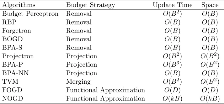
In contrast to the above approaches, our work explores a completely different approach, i.e., kernel functional approximation techniques, for resolving budget online kernel learning tasks. As a summary, Table 1 compares the properties of different budget online kernel
learning algorithms, including the proposed FOGD and NOGD algorithms, whereB is the
budget on the desired SV size,Dis the number of Fourier components, andkis the matrix
approximation rank of Nystr¨om.
Algorithms Budget Strategy Update Time Space
Budget Perceptron Removal O(B2) O(B)
RBP Removal O(B) O(B)
Forgetron Removal O(B) O(B)
BOGD Removal O(B) O(B)
BPA-S Removal O(B) O(B)
Projectron Projection O(B2) O(B2)
BPA-P Projection O(B3) O(B2)
BPA-NN Projection O(B) O(B)
TVM Merging O(B2) O(B2)
FOGD Functional Approximation O(D) O(D)
NOGD Functional Approximation O(kB) O(kB)
Table 1: Comparison on different budget online kernel learning algorithms.
Moreover, our work is also related to kernel methods for classification tasks (Shawe-Taylor and Cristianini, 2004; Hoi et al., 2006, 2007), especially for some studies on large-scale kernel methods (Williams and Seeger, 2000; Rahimi and Recht, 2007). Our approach shares the similar idea with the Low-rank Linearization SVM (LLSVM) (Zhang et al., 2012), where the non-linear SVM is transformed into a linear problem via kernel approximation meth-ods. Unlike their approach, we employ the technique of random Fourier features (Rahimi and Recht, 2007), which have been successfully explored for speeding up batch kernelized SVMs (Rahimi and Recht, 2007; Yang et al., 2012) and kernel-based clustering (Chitta et al., 2011, 2012) tasks. Besides, another kernel approximation technique used in our approach
is the well-known Nystr¨om method (Williams and Seeger, 2000), which has been widely
3. Large Scale Online Kernel Learning for Binary Classification
In this section, we introduce the problem formulation of online kernel binary classification and the detailed steps of our proposed algorithms.
3.1 Problem Formulation
We consider the problem of online learning for binary classification by following online
convex optimization settings. Our goal is to learn a functionf :Rd→Rfrom a sequence of
training examples{(x1, y1), . . . ,(xT, yT)}, where instance xt∈Rd and class labelyt∈ Y =
{+1,−1}. We refer to the output f of the learning algorithm as a hypothesis and denote
the set of all possible hypotheses byH={f|f :Rd→R}. We will use `(f(x);y) :R2 →R
as the loss function that penalizes the deviation of estimating f(x) from observed labels
y. Further, we considerH a Reproducing Kernel Hilbert Space (RKHS) endowed with a
kernel function κ(·,·) : Rd×Rd → R (Vapnik, 1998) implementing the inner producth·,·i
such that: 1) κ has the reproducing property hf, κ(x,·)i = f(x) for x ∈ Rd; 2) H is the
closure of the span of allκ(x,·) withx∈Rd, that is,κ(x,·)∈ H ∀x∈ X. The inner product
h·,·i induces a norm on f ∈ H in the usual way: kfkH := hf, fi
1
2. To make it clear, we
denote byHκ an RKHS with explicit dependence on kernelκ. Throughout the analysis, we
assume κ(xi,xj)≤1,∀xi,xj ∈Rd.
Training an SVM classifierf(x) can be formulated as the following optimization problem
min
f∈Hκ
P(f) = λ 2kfk
2 H+
1
T
T X
t=1
`(f(xt);yt),
where λ >0 is a regularization parameter used to control model complexity. While in an
pure online setting, the regularized loss in thet-th iteration is
Lt(f) =
λ
2kfk
2
H+`(f(xt);yt).
The goal of an online learning algorithm is to find a sequence of functions ft,t∈[T] that
achieve the minimumRegret along the whole learning process. The regret is defined as,
Regret=
T X
t=1
Lt(ft)− T X
t=1
Lt(f∗),
where f∗ = arg minfPTt=1Lt(f) is the optimal classifier assuming that we had foresight
in all the training instances. In a typical online budgeted kernel learning algorithm, the algorithm learns the kernel-based predictive modelf(x) for classifying a new instancex∈Rd
as follows:
f(x) =
B X
i=1
αiκ(xi,x),
where B is the number of Support Vectors (SV’s), αi denotes the coefficient of the i-th
approach aims to bound the number of SV’s by a budget constantB using different budget maintenance strategies. Unlike the existing budget online kernel learning methods using the budget maintenance strategies, we propose to tackle the challenge by exploring a completely different strategy, i.e., the kernel functional approximation approach that construct a
kernel-induced new representationz(x)∈RD such that the inner product of instances in the new
space is able to approximate the kernel function:
κ(xi,xj)≈z(xi)>z(xj).
By the above approximation, the predictive model can be rewritten:
f(x) =
B X
i=1
αiκ(xi,x)≈ B X
i=1
αiz(xi)>z(x) =w>z(x),
wherew=PBi=1αiz(xi) denotes the weight vector to be learned in the new feature space.
As a consequence, solving the regular online kernel classification task can be turned into a problem of an linear online classification task on the new feature space derived from the kernel approximation. In the following, we will present two online kernel learning algorithms for classification by applying two different kernel approximation methods: (i) Fourier Online
Gradient Descent (FOGD) and (ii) Nystr¨om Online Gradient Descent (NOGD) methods.
3.2 Fourier Online Gradient Descent
Random Fourier features can be used in shift-invariant kernels (Rahimi and Recht, 2007). A shift-invariant kernel is the kernel that can be written as κ(x1,x2) =k(∆x), wherek is
some function and ∆x=x1−x2 is the shift between the two instances. Examples of
shift-invariant kernels include some widely used kernels, such as Gaussian and Laplace kernels. By performing an inverse Fourier transform of the shift-invariant kernel function, one can obtain:
κ(x1,x2) =k(x1−x2) =
Z
p(u)eiu>(x1−x2)du, (1)
where p(u) is a proper probability density function calculated from the Fourier transform
of function k(∆x),
p(u) = ( 1 2π)
dZ e−iu>(∆x)
k(∆x)d(∆x). (2)
More specifically, for a Gaussian kernel κ(x1,x2) = exp(−
kx1−x2k2 2
2σ2 ), we have the
corre-sponding random Fourier component u with the distribution p(u) =N(0, σ−2I). And for
a Laplacian kernel κ(x1,x2) = exp(−
||x1−x2||1
σ ), we have p(u) = σΠd
1
π(1+σ2u2 d)
. Given a kernel function that is continuous and positive-definite, according to the Bochner’s theo-rem (Rudin, 1990), the kernel function can be expressed as an expectation of function with
a random variableu:
Z
p(u)eiu>(x1−x2)du= Eu[eiu >x1
·e−iu>x2] (3)
= Eu[cos(u>x1) cos(u>x2) + sin(u>x1) sin(u>x2)]
The equality (1) can be obtained by only keeping the real part of the complex function. From (3), we can see any shift-invariant kernel function can be expressed by the expectation of the inner product of the new representation of original data, where the new data repre-sentation is z(x) = [sin(u>x),cos(u>x)]>.As a consequence, we can sample D number of
random Fourier componentsu1, ...uD independently for constructing the new representation
as follows:
z(x) = (sin(u>1x),cos(u>1x), ...,sin(u>Dx),cos(u>Dx))>.
The online kernel learning task in the original input space can thus be approximated by solving a linear online learning task in the new feature space. For data arriving sequentially, we can construct the new representation of a data instance the-fly, and then perform on-line learning in the new feature space using the onon-line gradient descent algorithm. We refer to the proposed algorithm as the Fourier Online Gradient Descent (FOGD), as summarized in Algorithm 1.
3.3 Nystr¨om Online Gradient Descent
The above random Fourier feature based approach attempts to approximate the kernel function explicitly, which is in general data independent for the given dataset and thus may not fully exploit the potential of data distribution for kernel approximation. To address this,
we propose to explore the Nystr¨om method (Williams and Seeger, 2000) to approximate a
large kernel matrix by a data-dependent approach.
Before presenting the method, we first introduce some notations. We denote a kernel
matrix by K ∈ RT×T with rank r, the Singular Value Decomposition (SVD) of K as
K=VDV>, where the columns ofVare orthogonal andD= diag(σ1, . . . , σr,) is diagonal.
For k < r,Kk =
Pk
i=1σiViVi> =VkDkV>k is the best rank-k approximation of K, where
Vi is the i-th column of matrix V.
Given a large kernel matrixK∈RT×T, the Nystr¨om method randomly samplesB T
columns to form a matrix C∈RT×B, and then derive a much smaller kernel matrixW ∈
RB×B based on the sampled B instances. We can in turn approximate the original large
kernel matrix by
ˆ
K=CW+kC>≈K, (4)
whereWkis the best rank-kapproximation ofW,W+denotes the pseudo inverse of matrix
W.
We now apply the above Nystr¨om based kernel approximation to tackle large-scale online
kernel classification task. Similar to the previous approach, the key idea is to construct the new representation for every newly arrived data instance based on the kernel approximation principle. In particular, we propose the following scheme: (i) at the very early stage of the online classification task, we simply run any existing online kernel learning methods (e.g., kernel-based online gradient descent in our approach) whenever the number of SV’s
is smaller than the predefined budget B; (ii) once the budget is reached, we then use the
storedB SV’s to approximate the kernel value of any new instances (which is equivalent to
using the firstB columns to approximate the whole kernel matrix). From the approximated
Algorithm 1 FOGD — Fourier Online Gradient Descent for Binary Classification
Input: the number of Fourier componentsD, step size η, kernel functionk;
Initialize w1 = 0.
Calculate p(u) for kernelk as (2).
Generate random Fourier components: u1, ...,uD sampled from distribution p(u)
for t= 1,2, . . . , T do
Receivext;
Construct new representation:
zt(xt) = (sin(u>1xt),cos(u>1xt), ...,sin(u>Dxt),cos(u>Dxt))>
Predictybt= sgn(w>t z(xt));
Receiveyt and suffer loss` w>t z(xt);yt
;
if ` w>t z(xt);yt
>0 then wt+1 =wt−η∇` wt>z(xt);yt
.
end if end for
Algorithm 2 NOGD — Nystr¨om Online Gradient Descent for Binary Classification
Input: the budget B, step size η, rank approximation k.
Initialize support vector setS1 =∅, and model f1= 0. while |St|< B do
Receive new instancext;
Predictybt= sgn(ft(xt));
Updateft by regular Online Gradient Descent (OGD);
UpdateSt+1 =St∪ {t}whenever loss is nonzero;
t=t+ 1;
end while
Construct the kernel matrix ˆKt from St.
[Vk,Dk] =eigs( ˆKt, k), where Vk and Dk are Eigenvectors and Eigenvalues of ˆKt.
Initialize w>t = [α1, ..., αB](D−0k .5Vk>)−1.
Initialize the instance index T0=t; for t=T0, . . . , T do
Receive new instancext;
Construct the new representation ofxt:
z(xt) =Dk−0.5Vk>(κ(xt,xˆ1), ..., κ(xt,xˆB))>.
Predictybt= sgn(w>t z(xt));
Updatewt+1 =wt−η∇` w>t z(xt);yt
.
xj is approximated by the following
ˆ
κ(xi,xj) = (CiVkD
−1 2
k )(CjVkD
−1 2
k )
>
= ([κ(ˆx1,xi), ..., κ(ˆxB,xi)]VkD
−1 2
k )(κ(ˆx1,xj), ..., κ(ˆxB,xj)VkD
−1 2
k )
>,
where ˆxa, a∈ {1, ..., B} is the a-th support vector.
For a new instance, we construct the new representation as follows:
z(x) = ([κ(ˆx1,x), ..., κ(ˆxB,x)]VkD
−1 2
k )
>.
Similarly, we can then apply the existing online gradient descent algorithm to learn the
linear predictive model on the new feature space induced from the kernel. We denote
the proposed algorithm the Nystr¨om Online Gradient Descent (NOGD), as summarized
in Algorithm 2. Different from the FOGD algorithm, the algorithm follows the kernelized online gradient descent until the number of SV’s reachesB. To initialize the linear classifier
w, we aim to achieve
w>z(x) = [α1, ..., αB][κ(ˆx1,x), ..., κ(ˆxB,x)]>,
thus
w>D−
1 2
k V
>
k[κ(ˆx1,x), ..., κ(ˆxB,x)]>= [α1, ..., αB][κ(ˆx1,x), ..., κ(ˆxB,x)]>.
The solution is
w>D−
1 2
k V
>
k = [α1, ..., αB];
w>= [α1, ..., αB](D
−1 2
k V
>
k)
−1 .
4. Theoretical Analysis
In this section, we analyze the theoretical properties of the two proposed algorithms. We may use `t(f) instead of `(f(xt);yt) for simplicity.
Theorem 1 Assume we have a shift-invariant kernel κ(x1,x2) = k(x1 −x2), where k
is some function and the original data is contained by a ball Rd of diameter R. Let `(f(x);y) : R2 → R be a convex loss function that is Lipschitz continuous with Lipschitz constant L. Let wt, t ∈ [T] be the sequence of classifiers generated by FOGD in
Algo-rithm 1. Then, for any f∗(x) =PT
t=1α
∗
tκ(x,xt), we have the following with probability at
least 1−28(σpR )2exp(4(−dD+2)2 ),
T X
t=1
`t(wt)− T X
t=1
`t(f∗)≤
(1 +)kf∗k2 1
2η +
η
2L
2T+LTkf∗k 1,
where kf∗k1 = PTt=1|α∗t|, σp2 = Ep[u>u] is the second moment of the Fourier transform
Proof Given f∗(x) = PTt=1α∗tκ(x,xt), according to the representer theorem (Sch¨olkopf
et al., 2001), we have a corresponding linear model: w∗ =PTt=1α∗tz(xt), where
z(x) = (sin(u>1x),cos(u>1x), ...,sin(u>Dx),cos(u>Dx))>.
The first step to prove our theorem is to bound the regret of our sequence of linear model
wt learned by our online learner with respect to the linear model w∗ in the new feature
space. First of all, we have the following:
kwt+1−w∗k2 =kwt−η∇`t(wt)−w∗k2
=kwt−w∗k2+η2k∇`t(wt)k2−2η∇`t(wt)(wt−w∗).
Combining the above and the convexity of the loss function, i.e.,
`t(wt)−`t(w∗)≤ ∇`t(wt)(wt−w∗),
we then have the following
`t(wt)−`t(w∗)≤
kwt−w∗k2− kwt+1−w∗k2
2η +
η
2k∇`t(wt)k
2.
Summing the above overt= 1, ..., T leads to:
T X
t=1
(`t(wt)−`t(w∗)) ≤
kw1−w∗k2− kwT+1−w∗k2
2η +
η
2
T X
t=1
k∇`t(wt)k2
≤ kw ∗k2
2η +
η
2L
2T. (5)
Next we further examine the relationship betweenPTt=1`t(w∗) andPTt=1`t(f∗). According
to the uniform convergence of Fourier features (Claim 1 in Rahimi and Recht (2007)), we have the high probability bound for the difference between the approximated kernel value and the true kernel value, i.e., with probability at least 1−28(σpR )2exp(4(−dD+2)2 ), where
σp2 =Ep[u>u] is the second moment of the Fourier transform of the kernel functionkgiven
thatp(u) is the probability density function calculated by the Fourier transform of function
k. We have ∀i, j
|z(xi)>z(xj)−κ(xi,xj)|< .
Since we assumeκ(xi,xj)≤1, we can assume z(xi)>z(xj)≤1 +, which lead to:
kw∗k2 ≤(1 +)kf∗k21. (6) When |z(xi)>z(xj)−κ(xi,xj)|< , we have
|
T X
t=1
`t(w∗)− T X
t=1
`t(f∗)| ≤ T X
t=1
|`t(w∗)−`t(f∗)|
≤
T X
t=1
L
T X
i=1
|α∗i||z(xi)>z(xt)−κ(xi,xt)|
≤
T X
t=1
L
T X
i=1
Combining (5), (6) and (7) leads to complete the proof.
Remark 1. In general, the larger the dimensionality D, the higher the probability of the bound to be achieved. This means that by sampling more random Fourier components, one can approximate the kernel function more accurately and effectively. From the above theorem, it is not difficult to show that, by settingη= √1
T and =
1 √
T, we have
T X
t=1
`t(wt)− T X
t=1
`t(f∗) ≤ (
2kf∗k1+L2
2 +Lkf
∗k 1)
√
T ,
which leads to a sub-linear regretO(√T). However, setting= √1
T requires to sampleD=
O(T) random components in order to achieve a high probability, which seems unsatisfactory
since we will have to solve a very high-dimensional linear online learning problem. However, even in this case, for our FOGD algorithm, the learning time cost for each instance is
O(c1T), while the time cost for classifying an instance by regular online kernel classification
is O(c2T), here c1 is the time for a scalar product by FOGD, while c2 is the time for
computing the kernel function. Since c2 c1, our method is still much faster than the
regular online kernel classification methods.
Remark 2. This theorem bounds the regret for any shift-invariant kernel. Specially, we can get the bound for a Gaussian kernelk(x1−x2) = exp(−γ||x1−x2||2), by settingσp2 = 2dγ
(Rahimi and Recht, 2007).
The theoretical analysis for the NOGD algorithm follows the similar procedure as used by the FOGD algorithm. We first introduce a lemma to facility our regret bound analysis.
Lemma 1 P(f) = λ2kfk2 H+ T1
PT
t=1`t(f) is the objective function of an SVM problem,
where `t(f) is the hinge loss function of the t-th iteration. Define f∗ to be the optimal
solution when using the exact kernel matrix K and fN as the optimal when adopting the
Nystr¨om approximated kernel matrix Kˆ. We have
P(fN)−P(f∗)≤
1
2T λ||K−
ˆ
K||2,
where kK−Kˆk2 is the spectral norm of the kernel approximation gap.
This lemma mainly follows the Lemma 1 in (Yang et al., 2012), we omit the proof for conciseness.
Theorem 2 Assume we learn with kernelκ(xi,xj)≤1, ∀i, j ∈[T]. Let`(f(x);y) :R2 → R be the hinge loss function. Let the sequence of T instances x1, ...,xT form a kernel
matrix K∈ RT×T, and Kˆ is the approximation of K using Nystr¨om method. Let f
t(x) =
w>tz(x), t ∈ [T] be the sequence of classifiers generated by NOGD in Algorithm 2. We assume the norm of the gradients in all iterations are always bounded by a constant L, which is easy to achieve by a few projection steps when necessary. In addition, define fN(x) = w>Nz(x) be the optimal classifier when using Nystr¨om kernel approximation and
original kernel space with the assumption of the foresight for all the instances, we have the following:
T X
t=1
Lt(wt)− T X
t=1
Lt(f∗)≤
kwNk2
2η +
η
2L
2T+ 1
2λ||K−
ˆ
K||2.
Proof Following the similar analysis as in Theorem 1, the regularized loss function in the
t-th iteration,Lt(w) = λ2||w||22+`t(w) satisfies the following bound, T
X
t=1
(Lt(wt)− Lt(wN))≤
kwNk2
2η +
η
2L
2T.
As proven in (Yang et al., 2012), the linear optimization problem in z(x) space, i.e.,
P(w) = λ2||w||2 2+T1
PT
t=1`t(w) is equivalent to the approximated SVMP(f) =
λ
2||f|| 2 H+ 1
T PT
t=1`t(f) when f ∈ HN is the functional space of Nystr¨om method. From Lemma 1,
we have,
T X
t=1
Lt(wN) = T X
t=1
Lt(fN) =T P(fN)≤T P(f∗) +
1
2λ||K−Kˆ||2 =
T X
t=1
L(f∗) + 1
2λ||K−Kˆ||2.
We complete the proof by combining the above two formulas.
Remark. As shown in Theorem 5 of (Yang et al., 2012), the kernel approximation gap
||K−Kˆ||2≤O(TB). Consequently when settingB = √
T and η= √1
T, we have
T X
t=1
Lt(wt)− T X
t=1
L(f∗)≤O(
√
T).
This theorem bounds the regret of the NOGD algorithm when using all singular values
of matrix W but only O(√T) support vectors. However, when the rank of the Nystr¨om
approximated matrix ˆK is only k, the bound should be slightly worse. As (Cortes et al.,
2010)(Theorem 1) shows, the following holds with probability at least 1−,
kKˆ −Kk2 ≤ kK−Kkk2+ T
√
BKmax(2 + log
1
),
where kK−Kkk2 is the spectral norm of the best rank-k approximated gap and Kmax is
the maximum diagonal entry ofK. This indicates that to get theO(√T) regret bound, we
should set the budget sizeB =T /c, wherecis some constant. This seems suboptimal, but
we will demonstrate that only a small budget size is needed for satisfactory performance in
our experimental results. In addition, the time cost of using k-rank approximation is only
k/B times of that when using all singular values, which makes the algorithm extremely
5. Large Scale Online Kernel Learning for Multi-class Classification
In this section, we extend the proposed Fourier Online Gradient Descent and Nystr¨om
Online Gradient Descent methods, which are originally designed for binary classification, to online multi-class classification task. We also give theoretical analysis of the two approaches.
5.1 Problem Settings
Similar to online binary classification tasks, online multi-class classification is performed over a sequence of training examples (xt, yt), t = 1, . . . , T, where xt ∈ Rd is the observed
features of the t-th training instance. Unlike binary classification where class label yt ∈
Y ={+1,−1}, in a multi-class classification task, each label belongs to a finite setY of size
m >2, i.e.,yt∈ Y ={1, . . . , m}. The true class labelytis only revealed after the prediction
ˆ
yt∈ Y is made.
We follow the protocol of multi-prototype classification for deriving multi-class online
learning algorithm (Crammer et al., 2006). Specifically, it learns a function fr :Rd→ R
for each of the classes r ∈ Y. During the t-th iteration, the algorithm predicts a sequence of scores for the classes:
ft1(xt), . . . , ftm(xt)
.
The predicted class is set to be the class with the highest prediction score:
ˆ
yt= arg max
r∈Y
ftr(xt). (8)
We then define st as the irrelevant class with the highest prediction score:
st= arg max r∈Y,r6=yt
ftr(xt).
The margin with respect to the hypothesis in the t-th iteration is defined to be the gap
between the prediction score of class yt andst:
γt=ftyt(xt)−ftst(xt).
Obviously, in a correct prediction, the margin γt > 0. However, as stated in (Crammer
et al., 2006), we are not satisfied by a positive margin value and thus we define ahinge-loss function:
` ft,xt, yt
= max(0,1−γt),
whereft denotes the set of allm functions for all classes.
5.2 Multi-class Fourier Online Gradient Descent
As introduced in the previous section for binary classification task, the online multi-class kernel classification task in the original input space can also be approximated by solving a linear online learning task in the new feature space. First, we use the same Fourier feature
mapping approach as in the binary case to map each input instance xt to z(xt). Then
Following the multi-class problem setting, we learn a weight vectorwr ∈Rdfor each of
the classes r∈ Y. And use the linear classifierfr(xt) =wr·z(xt) to approximate to kernel
prediction score. During the t-th iteration, the algorithm predicts a sequence of scores for them classes:
w1t ·z(xt), . . . ,wmt ·z(xt)
.
We define the hinge-loss function as following:
` wt,xt, yt
= max(0,1−γt) = max(0,1−wytt ·z(xt) +wstt ·z(xt)), (9)
wherewt denotes the set of allm weight vectors.
Following the Online Gradient Descent approach, the update strategy ofwtwhen` >0
is:
wtr+1=wtr−η∇` wt,xt, yt
,
whereη is a positive learning rate parameter and the gradient is taken with regards towtr. By rewriting the loss function explicitly, we can rewrite the above as follows:
wytt+1=wytt +ηz(xt); (10)
wstt+1=wstt −ηz(xt). (11)
Only two of the weight vectors are updated during each iteration. Thus, we can derive the FOGD algorithm for multi-class versions, as summarized in Algorithm 3.
5.3 Multi-class Nystr¨om Online Gradient Descent
Similar to the binary task, in the first a few iterations of multi-class online Nystr¨om
algo-rithm (before the size of SV set reaches the predetermined budget size B), the algorithm
performs a regular Online Gradient Descent update to them kernel classifiers when` >0:
ftr+1 =ftr−η∇` ft,xt, yt
,
where η >0 is the gradient descent step size and the gradient is taken with regard to ftr. By rewriting the loss function explicitly, we have
ftyt+1=ftyt +ηκ(xt,·); (12)
ftst+1 =ftst −ηκ(xt,·). (13)
Therefore, we need to store a SV setS and update it when necessary: St+1 =St∪ {t}. Note
that all them classifiers share the same SV set, which is the same setting as that of binary case. However, the storage strategy for αi, i.e., the coefficient of the i-th SV, is different
from that of binary case. In multi-class task, a vector αi ∈ Rm is used to represent the
coefficients of the i-th SV. Each of its element αri is the coefficient of the i-th SV for the kernel classifier fr. Obviously,αri = 0 if r =6 yt and r6=st.
After the size of SV set reaches the budget B, we do a Nystr¨om feature mapping as the
approach discussed in the binary section to map each input instancexttoz(xt). The
follow-ing linear update steps follow that in the multi-class Fourier Gradient Descent algorithm, as equation (10) and (11).
Algorithm 3 MFOGD — Multi-class Fourier Online Gradient Descent
Input: the number of Fourier componentsD, step size η, kernel functionk;
Initialize w1r= 0,r = 1, ..., m. Calculate p(u) for kernelk as (2).
Generate random Fourier components: u1, ...,uD sampled from distribution p(u).
for t= 1,2, . . . , T do
Receivext;
Construct new representation:
z(xt) = (sin(u>1xt),cos(u>1xt), ...,sin(u>Dxt),cos(u>Dxt))>
Predict as in (8);
Receiveyt and suffer loss` wt,xt, yt
(9);
if ` wt,xt, yt
>0 then
updatewt as (10) and (11)
end if end for
Algorithm 4 MNOGD — Multi-class Nystr¨om Online Gradient Descent
Input: the budget B, step size η, rank approximation k.
Initialize support vector setS1 =∅, and model f1r = 0,r= 1, ..., m.
while |St|< B do
Receivext;
Predict as in (8);
Updateft by regular Online Gradient Descent (OGD), as (12) and (13);
UpdateSt+1 =St∪ {t}whenever loss is nonzero;
t=t+ 1;
end while
Construct the kernel matrix ˆKt from St.
[Vk,Dk] =eigs( ˆKt, k), where Vk and Dk are Eigenvectors and Eigenvalues of ˆKt.
Initialize wrt>= [αr1, ..., αrB](Dk−0.5Vk>)−1,r= 1, ..., m. Initialize the instance index T0=t;
for t=T0, . . . , T do
Receivext;
Construct the new representation ofxt:
z(xt) =Dk−0.5Vk>(κ(xt,xˆ1), ..., κ(xt,xˆB))>.
Predict as in (8);
Updatewt as (10) and (11)
5.4 Theoretical Analysis
In this section, we analyze the theoretical properties of the two proposed multi-class algo-rithms. We may use`t(f) instead of`(f ,xt, yt) for simplicity.
Theorem 3 Assume we have a shift-invariant kernel κ(x1,x2) = k(x1−x2), where k is
some function and the original data is contained by a ball Rd of diameterR. Let` f ,x, y be the hinge-loss we talked above, wheref denotes the set of m classifiers for them classes and its output is a sequence of prediction scores. Let wt, t ∈ [T] be the sequence of
clas-sifiers generated by MFOGD in Algorithm 3. Then, for any f∗r(x) = PTt=1αrt∗κ(x,xt),
r∈ {1, ..., m}, we have the following with probability at least 1−28(σpR )2exp(4(−dD+2)2 )
T X
t=1
`t(wt)− T X
t=1
`t(f∗)≤
m(1 +)kf∗k21
2η +ηT D+ 2T kf∗k1,
where kf∗k1 =PTt=1maxr∈Y|αtr∗|, and σ2p =Ep[u>u]is the second moment of the Fourier
transform of the kernel function kgiven that p(u) is the probability density function calcu-lated by the Fourier transform of function k.
Proof Given f∗r(x) = PTt=1αr ∗
t κ(x,xt), r = 1, ...m, according to the Representer
Theo-rem (Sch¨olkopf et al., 2001), we have a corresponding linear model: wr∗ = PTt=1αr ∗
t z(xt),
where
z(x) = (sin(u>1x),cos(u>1x), ...,sin(u>Dx),cos(u>Dx))>.
The first step to prove our theorem is to bound the regret of the sequence of linear models
wtlearned by online learner with respect to the linear model w∗ in the new feature space.
We first have
kwrt+1−wr∗k2− kwtr−wr∗k2 = kwtr−w∗r+βtrz(xt)k2− kwrt −wr∗k2
= (βrt)2kz(xt)k2+ 2βtr(wrt·z(xt)−wr∗·z(xt)),
where βtr is the parameter used to update wtr as (10) and (11). Thus, it may be η, −η, or 0. Obviously, kz(xt)k2 =D. We first assume that`t(wt)>0 and there are updates in the
t-th iteration. Summing the above overr = 1, ..., m, we have
m X
r=1
kwtr+1−w∗rk2− kwrt−w∗rk2
= 2η2D+ 2η(wytt ·z(xt)−wstt ·z(xt))−2η(wyt∗ ·z(xt)−wst∗ ·z(xt)),
where yt is the true label in the t-th iteration and st is the label of the largest scored
irrelevant label classified by the classifier setwt, not by the classifier setw∗. Thus we have:
wytt ·z(xt)−wstt ·z(xt) =γw,t w∗yt ·z(xt)−wst∗ ·z(xt)≥γw∗,t.
As we have assumed `t(wt) > 0, we have `t(wt) = 1−γw,t. And from the fact that
`t(w∗)≥1−γw∗,t, we have:
Combining the three formula above, we get
`t(wt)−`t(w∗)≤ηD+
Pm
r=1kwrt−w∗rk2−Pmr=1kwrt+1−wr∗k2
2η .
Note that in some iterations, `t(wt) = 0 and there is no update in the t-th iteration, i.e.,
wr
t = wrt+1. The above formula still holds. Summing it over t = 1, ...T and assuming
wr1= 0 for all r= 1, ..., mleads to:
T X
t=1
`t(wt)− T X
t=1
`t(w∗)≤ηT D+
Pm
r=1kwr∗k2
2η . (14)
Next we further examine the relationship betweenPTt=1`t(w∗) andPTt=1`t(f∗). According
to the uniform convergence of Fourier features (Claim 1 in Rahimi and Recht (2007)), we have the high probability bound for the difference between the approximated kernel value and the true kernel value, i.e., with probability at least 1−28(σpR
)2exp(
−D2
4(d+2)), where σp2 =Ep[u>u] is the second moment of the Fourier transform of the kernel functionkgiven
thatp(u) is the probability density function calculated by the Fourier transform of function
k. We have ∀i, j
|z(xi)>z(xj)−κ(xi,xj)|< .
Similar to the binary case:
m X
r=1
kwr∗k2≤mkf∗k21(1 +). (15)
When |z(xi)>z(xj)−κ(xi,xj)|< , we have
|
T X
t=1
`t(w∗)−
T X
t=1
`t(f∗)| ≤
T X
t=1
|`t(w∗)−`t(f∗)| ≤
T X
t=1
L|γw∗,t−γf∗,t|
= T X t=1 | T X i=1
(αyti ∗z(xi)>z(xt)−αsti ∗z(xi)>z(xt))− T X
i=1
(αyti ∗κ(xi,xt)−α s0t∗
i κ(xi,xt))|
≤ T X t=1 T X i=1
|αyti ∗z(xi)>z(xt)−αyti ∗κ(xi,xt)|+ T X
i=1
|αsti ∗z(xi)>z(xt)−αs 0 t∗
i κ(xi,xt)|
,
whereLin the first line is the Lipschitz constant and can be set to 1 in hinge loss case, and
st is the largest scored irrelevant label with regards to w∗ and s0t with regard tof∗. Thus
the bound of the first term is easy to find and we will focus on the second term. Without loss of generality, we assume αsti ∗z(xi)>z(xt) ≥ αs
0 t∗
i κ(xi,xt). According to the definition
of st and s0t,α s0t∗
i κ(xi,xt)> α st∗
i κ(xi,xt), leading to:
|αsti ∗z(xi)>z(xt)−αs 0 t∗
i κ(xi,xt)| ≤ |α st∗
i z(xi)
>z(x
t)−κ(xi,xt)
Consequently, we have
|
T X
t=1
`t(w∗)−
T X
t=1
`t(f∗)| ≤2T kf∗k1. (16)
Combining (14), (15) and (16) leads to complete the proof.
Similar to the analysis of the binary classification case, it is not difficult to observe that
the proposed MFOGD algorithm also achieves sub-linear regret O(√T). We will continue
the analysis of MNOGD method in the following. As in the binary analysis, we first pro-pose a lemma that bounds the gap of averaged loss between the exact kernel SVM and approximated kernel SVM. Unlike the binary classification problem, there are many differ-ent problem settings for the multi-class SVM problem, as surveyed by Hsu and Lin (2002). For consistency, in the following analysis, we adopt the common slack variables for all classes setting (Crammer and Singer, 2001, 2002).
Lemma 2 P(f) = λ2Pmr=1kfrk2 H+T1
PT
t=1`t(f)is the objective function of an multi-class
SVM problem, where`t(f)is the multi-class hinge loss function of thet-th iteration. Define
f∗ as the optimal solution of P(f) when using the exact kernel matrix K and f
N as the
optimal solution of SVM algorithm when adopting the Nystr¨om approximated kernel matrix ˆ
K. We have
P(fN)−P(f∗)≤
m
2T λ||K−Kˆ||2,
where kK−Kˆk2 is the spectral norm of the kernel approximation gap. Proof The dual problem of multi-class SVM is
maxP(α) =− 1
2λ
m X
r=1
α>rKαr−
m X
r=1
α>rer,
s.t.
m X
r=1
αt,r= 0, ∀t∈ {1,2, ..., T};
αt,r ≤0, ifyt6=r, αt,r≤
1
T,ifyt=r, ∀t∈ {1,2, ..., T}, ∀r∈ {1,2, ...m}
where αr = [α1,r, α2,r, ..., αT ,r]>, er = [e1,r, e2,r, ..., eT,r]> and et,r = 0 if yt =r, otherwise
et,r= 1.
We can get the dual problem of the Nystr¨om approximated multi-class SVM by replacing
the kernel matrix Kwith ˆK.
P(fN) = max " − 1 2λ m X r=1
α>rKˆαr−
m X
r=1
α>rer # = max " − 1 2λ m X r=1
α>r( ˆK−K+K)αr−
m X
r=1
α>rer # = max " 1 2λ m X r=1
α>r(K−Kˆ)αr # + max " − 1 2λ m X r=1
α>rKαr−
m X
r=1
α>rer #
Consequently,
P(fN)−P(f∗)≤max
1 2λ
m X
r=1
α>r(K−Kˆ)αr≤max
m X
r=1
1 2λ||αr||
2
2||K−Kˆ||2.
We complete the proof by considering |αt,r| ≤ T1.
Theorem 4 Assume we learn with kernelκ(xi,xj)≤1,∀i, j∈[T]. Let`(f(x);y) :R2→R be the multi-class hinge loss function. Let the sequence of T instances x1, ...,xT form a
kernel matrix K∈ RT×T, and Kˆ is the approximation of K using Nystr¨om method . Let
ftr(x) =w>t,rz(x), t∈[T], r∈ {1,2, ..., m} be the sequence of classifiers generated by NOGD in Algorithm 4. We assume the norm of the gradients in all iterations are always bounded by a constant L, which is easy to achieve by a few projection steps when necessary. In addition, define fNr(x) = w>N,rz(x), r ∈ {1,2, ..., m} be the optimal classifier when using Nystr¨om kernel approximation and assuming we had foresight for all instances. By defining f∗ as the optimal classifier in the original kernel space with the assumption of the foresight for all the instances, we have the following:
T X
t=1
Lt(wt)− T X
t=1
Lt(f∗)≤
m X
r=1
kwN,rk2
2η +
η
2L
2T+ m
2λ||K−Kˆ||2.
This theorem is a combination of standard online gradient descent analysis and Lemma 2. The proof is omitted since it is similar to the binary analysis and straightforward. It’s easy to find that the multi-class NOGD algorithm enjoys the similar regret bound as the binary algorithm.
6. Large Scale Online Kernel Learning for Regression
In this section, we extend the proposed FOGD and NOGD algorithms to tackle online regression tasks. Consider a typical online regression task with a sequence of instances (xt, yt), t= 1, ..., T, wherext ∈ Rd is the feature vector of the t-th instance and yt ∈R is
the real target value, which is only revealed after the prediction is made at each iteration.
The goal of online kernel regression task is to learn a model f(x) that maps a new input
instance x∈Rd to a real value prediction:
f(x) =
B X
i=1
αiκ(xi,x).
We apply the squared loss as the evaluation metric of regression accuracy:
`(f(xt);yt) = (f(xt)−yt)2.
As the same approximation strategy with the previous task, with a feature mapping function
training instances. We use online gradient descent algorithm in this new feature space.
In order to reduce the frequency of update, we define as the threshold. Update is only
performed when the loss exceeds threshold. We denote the proposed algorithms the FOGD
for Regression (FOGD-R) and NOGD (NOGD-R) for regression tasks, as summarized in Algorithm 5 and Algorithm 6.
We omit the theoretical analysis of regression since it is similar to the binary case.
7. Experimental Results
In this section, we conduct an extensive set of experiments to examine the efficacy of the
proposed algorithms for several kinds of learning tasks in varied settings. Specifically,
our first experiment is to evaluate the empirical performance of the proposed FOGD and NOGD algorithms for regular binary classification tasks by following a standard batch learning setting where each dataset is divided into two parts: training set and test set. This experiment aims to make a direct comparison of the proposed algorithms with some state-of-the-art approaches for solving batch classification tasks.
Our second major set of experiments is to evaluate the effectiveness and efficiency of the proposed FOGD and NOGD algorithms for online learning tasks by following a purely online learning setting, where the performance measures are based on average mistake rate and time cost accumulated in the online learning process on the entire dataset (there is no split of training and test sets). In particular, we conduct such experiments for three different online learning tasks: binary classification, multi-class classification, and regression, by comparing the proposed algorithms with a variety of state-of-the-art budget online kernel learning algorithms.
All the source code and datasets for our experiments in this work can be downloaded
from our project web page:http://LSOKL.stevenhoi.org/. We are planning to release
our algorithms in the future release of the LIBOL library (Hoi et al., 2014).
7.1 Experiment for Binary Classification Task in Batch Setting
In this section, we compare our proposed algorithms with many state-of-the-art batch clas-sification algorithms. Different from online learning, the aim of a batch learning task is to train a classifier on the training dataset so that it achieves the best generalized accuracy on the test dataset.
7.1.1 Experimental Test bed and Setups
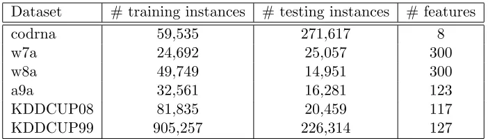
Table 2 summarizes the details of the datasets used in this experiment. All of them can
be downloaded from LIBSVM website 1 or KDDCUP competition site 2. We follow the
original splits of training and test sets in LIBSVM. For KDD datasets, a random split of 4/1 is used.
We compare the proposed algorithms with the following widely used algorithms for training kernel SVM for batch classification tasks:
1.http://www.csie.ntu.edu.tw/˜cjlin/libsvmtools/
Algorithm 5 FOGD-R — Fourier Online Gradient Descent for Regression
Input: the number of Fourier componentsD, step size η, threshold;
Initialize w1 = 0.
Calculate p(u) as (2). Generate random Fourier components:u1, ...,uD sampled from
distribution p(u).
for t= 1,2, . . . , T do
Receivext;
Construct new representation:
z(xt) = (sin(u>1xt),cos(u>1xt), ...,sin(u>Dxt),cos(u>Dxt))>
Predictybt=w>t z(xt);
Receiveyt and suffer loss` w>t z(xt);yt
;
if ` w>t z(xt);yt
> then wt+1 =wt−η∇` wt>z(xt);yt
.
end if end for
Algorithm 6 NOGD-R — Nystr¨om Online Gradient Descent for Regression
Input: the budget B, step size η, rank approximation k, threshold .
Initialize support vector setS1 =∅, and model f1= 0. while |St|< B do
Receive new instancext;
Predictybt=ft(xt);
Updateft by regular Online Gradient Descent (OGD);
UpdateSt+1 =St∪ {t}whenever loss exceeds threshold;
t=t+ 1;
end while
Construct the kernel matrix ˆKt from St.
[Vk,Dk] = eigs( ˆKt, k), where Vk and Dk are Eigenvectors and Eigenvalues of ˆKt,
re-spectively.
Initialize w>t = [α1, ..., αB](D−0k .5Vk>)−1.
Initialize the instance index T0=t; for t=T0, . . . , T do
Receive new instancext;
Construct the new representation of xt:
z(xt) =D−0k .5V
>
k(κ(xt,xˆ1), ..., κ(xt,xˆB))>.
Predictybt=w>t z(xt);
Update when loss exceeds: wt+1 =wt−η∇` w>t z(xt);yt
.
Dataset # training instances # testing instances # features
codrna 59,535 271,617 8
w7a 24,692 25,057 300
w8a 49,749 14,951 300
a9a 32,561 16,281 123
KDDCUP08 81,835 20,459 117
KDDCUP99 905,257 226,314 127
Table 2: Details of Binary Classification Datasets.
• “LIBSVM”: one of state-of-the-art implementation for batch kernel SVM available at
the LIBSVM website Chang and Lin (2011);
• “LLSVM”: Low-rank Linearization SVM algorithm that transfers kernel classification
to a linear problem using low-rank decomposition of the kernel matrix (Zhang et al., 2012);
• “BSGD-M”: The Budgeted Stochastic Gradient Descent algorithm which extends the
Pegasos algorithm (Shalev-Shwartz et al., 2011) by exploring the SV Merging strategy for budget maintenance (Wang et al., 2012b);
• “BSGD-R”: The Budgeted Stochastic Gradient Descent algorithm which extends the
Pegasos algorithm (Shalev-Shwartz et al., 2011) by exploring the SV Random Removal strategy for budget maintenance (Wang et al., 2012b).
To make a fair comparison of algorithms with different parameters, all the parameters,
including regularization parameter (C in LIBSVM, λ in pegasos), the learning rate (η in
FOGD and NOGD) and the RBF kernel width (σ) are optimized by following a standard
5-fold cross validation on the training datasets. The budget sizeB in NOGD and pegasos
algorithms and the feature dimensionDin FOGD are set individually for different datasets,
as indicated in the tables of experimental results. In general, these parameters are chosen such that they are roughly proportional to the size of support vectors output by the batch SVM algorithm in LIBSVM, since we would expect a relatively larger budget size for tackling
more challenging classification tasks in order to achieve competitive accuracy. The rank k
in NOGD is set to 0.2B for all datasets. For the online learning algorithms, all models
are trained by a single pass through the training sets and the reported accuracy and time cost are averaged over the five experiments conducted on different random permutations of the training instances. All the algorithms were implemented in C++, and conducted on a Windows machine with CPU of 3.0GHz. For the existing algorithms, all the codes can be
downloaded from LIBSVM website and BudgetedSVM website3.
7.1.2 Performance Evaluation Results
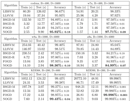
Table 3 shows the experimental results of batch binary classification tasks. We can drawn several observations from the results.
Algorithm codrna, B=400, D=1600 w7a, B=400, D=1600
Train (s) Test (s) Accuracy Train (s) Test (s) Accuracy
LIBSVM 80.20 126.02 96.67% 54.91 20.21 98.33%
LLSVM 19.04 37.34 95.93% 25.96 4.20 97.92%
BSGD-M 132.50 12.77 94.89%±0.41 37.41 3.91 97.50%±0.02
BSGD-R 3.32 12.77 67.16%±0.68 1.79 1.71 97.50%±0.01
FOGD 5.47 24.49 94.24%±0.22 1.58 1.46 97.59%±0.28
NOGD 2.55 9.90 95.92%±0.18 1.57 1.44 97.71%±0.09
Algorithm w8a, B=1000, D=4000 a9a, B=1000, D=4000
Train (s) Test (s) Accuracy Train (s) Test (s) Accuracy
LIBSVM 254.03 40.42 99.40% 97.81 24.80 85.04%
LLSVM 146.97 13.02 98.51% 70.85 14.43 84.89%
BSGD-M 230.51 2.42 97.52%±0.02 150.16 3.32 84.21%±0.18
BSGD-R 8.72 2.34 97.06%±0.04 7.03 3.28 81.96%±0.27
FOGD 13.04 3.85 97.93%±0.08 9.35 4.57 84.93%±0.03
NOGD 14.10 2.94 98.36%±0.10 16.94 3.37 84.99%±0.07
Algorithm KDD08, B=200, D=800 KDD99, B=200, D=400
Train (s) Test (s) Accuracy Train (s) Test (s) Accuracy
LIBSVM 1052.12 124.22 99.43% 20772.10 48.91 99.996%
LLSVM 24.31 3.53 99.38% 86.71 17.49 99.995%
BSGD-M 197.78 3.07 99.37%±0.01 948.21 12.11 99.994%±0.001
BSGD-R 12.34 3.03 99.12%±0.23 52.82 12.20 99.980%±0.031
FOGD 17.22 4.33 98.95%±3.34 26.81 6.80 99.996%± 0.001
NOGD 7.60 2.14 99.43%±0.04 20.71 9.03 99.993%±0.001
Table 3: Performance Evaluation Results on Batch Binary Classification Tasks.
First of all, by comparing the four online algorithms against the two batch algorithms, we found that the online algorithms in general enjoy significant advantage in terms of com-putational efficiency especially for large scale datasets. By further examining the learning accuracy, we found that some online algorithms, especially the proposed FOGD and NGOD algorithms, are able to achieve slightly lower but fairly competitive learning accuracy com-pared with the state-of-the-art batch SVM algorithm. This demonstrates that the proposed online kernel learning algorithms could be potentially a good alternative solution of the ex-isting SVM solvers when solving large scale batch kernel classification tasks in real-world applications due to their significant advantage of much lower learning time and memory costs.
(e.g., a9a, w7a and codrna), in which the difference between the number of support vectors of LIBSVM and the budget size is relatively larger than that of the other datasets. Thus, we can conclude that the high time cost of the BSGD-M(“pegasos+merging”) is due to the complex computation in the merging steps. Compared with the other online learning algo-rithms, the proposed NOGD algorithm achieves the highest accuracy for most cases while spending almost the lowest learning time cost. Similarly, FOGD algorithm also obtains more accurate result than the two budget Pegasos algorithms on most of the datasets with comparable or sometimes ever lower learning time cost. These facts indicate that the two proposed budget online kernel learning algorithms are both efficient and effective in solving large scale kernel classification problems.
Finally, by comparing the two proposed algorithms, we found that the performance of
NOGD is better than that of FOGD. This reflects that the Nystr¨om kernel approximation
tends to have a better approximation of the original RBF kernel than the Fourier feature based approximation.
7.2 Experiments for Online Binary Classification Tasks
In this section, we test the performance of our proposed algorithms on the online binary classification task.
7.2.1 Experimental Test beds and Setup
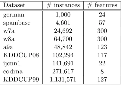
Table 4 shows the details of 9 publicly available datasets of diverse sizes for online binary classification tasks. All of them can be downloaded from LIBSVM website, UCI machine
learning repository 4 and KDDCUP competition site. As a yardstick for evaluation, we
Dataset # instances # features
german 1,000 24
spambase 4,601 57
w7a 24,692 300
w8a 64,700 300
a9a 48,842 123
KDDCUP08 102,294 117
ijcnn1 141,691 22
codrna 271,617 8
KDDCUP99 1,131,571 127
Table 4: Details of Online Binary Classification Datasets.
include the following two popular algorithms for regular online kernel classification without concerning budget:
• “Perceptron”: the kernelized Perceptron (Freund and Schapire, 1999) without budget;
• “OGD”: the kernelized online gradient descent (Kivinen et al., 2001) without budget.
Further, we compare the proposed budget online kernel learning algorithms with the fol-lowing state-of-the-art budget online kernel learning algorithms:
• “RBP”: the random budget perceptron by random removal strategy (Cavallanti et al.,
2007);
• “Forgetron”: the Forgetron by discarding oldest support vectors (Dekel et al., 2005);
• “Projectron”: the Projectron algorithm using the projection strategy (Orabona et al.,
2009);
• “Projectron++”: the aggressive version of Projectron algorithm (Orabona et al., 2008,
2009);
• “BPA-S”: the Budget Passive-Aggressive algorithm with simple SV removal strategy
in (Wang and Vucetic, 2010);
• “BOGD”: the Budget Online Gradient Descent algorithm by SV removal strategy
(Zhao et al., 2012);
To make fair comparisons, all the algorithms follow the same setups. We adopt the hinge
loss as the loss function `. Note that hinge loss is not a smooth function, whose gradient
is undefined at the point that the classification confidence yf(x) = 1. Following the sub-gradient definition, in our experiment, sub-gradient is only computed under the condition that
yf(x) < 1, and set to 0 otherwise. The Gaussian kernel bandwidth is set to 8. The step
sizeη in the all online gradient descent based algorithms is chosen through a random search
in range {2, 0.2, ..., 0.0002}. We adopt the same budget size B = 100 for NOGD and
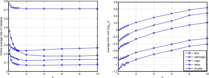
other budget algorithms. In the setting of FOGD algorithm,D=ρfB, where 0< ρf <∞
is a predefined parameter that controls the number of random Fourier components. For NOGD algorithm,k=ρnB, where 0< ρn <1 is a predefined parameter that controls the
accuracy of matrix approximation. We set ρf = 4 and ρn = 0.2 and will evaluate their
influence on the algorithm performance in the following discussion. For each data set, all the experiments were repeated 20 times using different random permutation of instances in the dataset. All the results were obtained by averaging over these 20 runs. For performance metrics, we evaluate the online classification performance by standard mistake rates and running time (seconds). All algorithms are implemented in Matlab R2013b, on a Windows machine with 3.0 GHZ CPU,6 cores.
7.2.2 Performance Evaluation Results
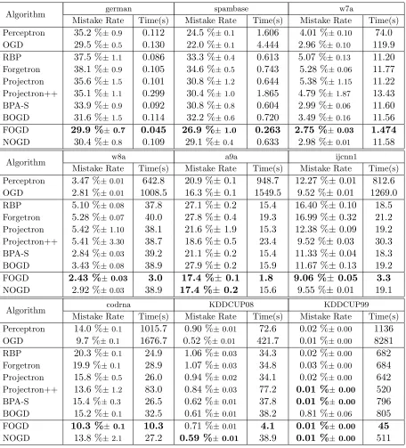
Table 5 summarizes the empirical evaluation results on the nine diverse data sets. From the results, we can draw the following observations.
Algorithm german spambase w7a
Mistake Rate Time(s) Mistake Rate Time(s) Mistake Rate Time(s)
Perceptron 35.2 %±0.9 0.112 24.5 %±0.1 1.606 4.01 %±0.10 74.0
OGD 29.5 %±0.5 0.130 22.0 %±0.1 4.444 2.96 %±0.10 119.9
RBP 37.5 %±1.1 0.086 33.3 %±0.4 0.613 5.07 %±0.13 11.20
Forgetron 38.1 %±0.9 0.105 34.6 %±0.5 0.743 5.28 %±0.06 11.77
Projectron 35.6 %±1.5 0.101 30.8 %±1.2 0.644 5.38 %±1.15 11.22
Projectron++ 35.1 %±1.1 0.299 30.4 %±1.0 1.865 4.79 %±1.87 13.43
BPA-S 33.9 %±0.9 0.092 30.8 %±0.8 0.604 2.99 %±0.06 11.60
BOGD 31.6 %±1.5 0.114 32.2 %±0.6 0.720 3.49 %±0.16 11.56
FOGD 29.9 %±0.7 0.045 26.9 %±1.0 0.263 2.75 %±0.03 1.474
NOGD 30.4 %±0.8 0.109 29.1 %±0.4 0.633 2.98 %±0.01 11.58
Algorithm w8a a9a ijcnn1
Mistake Rate Time(s) Mistake Rate Time(s) Mistake Rate Time(s)
Perceptron 3.47 %±0.01 642.8 20.9 %±0.1 948.7 12.27 %±0.01 812.6
OGD 2.81 %±0.01 1008.5 16.3 %±0.1 1549.5 9.52 %±0.01 1269.0
RBP 5.10 %±0.08 37.8 27.1 %±0.2 15.4 16.40 %±0.10 18.5
Forgetron 5.28 %±0.07 40.0 27.8 %±0.4 19.3 16.99 %±0.32 21.2
Projectron 5.42 %±1.10 38.1 21.6 %±1.9 15.3 12.38 %±0.09 19.2
Projectron++ 5.41 %±3.30 38.7 18.6 %±0.5 23.4 9.52 %±0.03 30.3
BPA-S 2.84 %±0.03 39.2 21.1 %±0.2 15.4 11.33 %±0.04 18.3
BOGD 3.43 %±0.08 38.9 27.9 %±0.2 15.9 11.67 %±0.13 19.2
FOGD 2.43 %±0.03 3.0 17.4 %± 0.1 1.8 9.06 %± 0.05 3.3
NOGD 2.92 %±0.03 38.9 17.4 %± 0.2 15.6 9.55 %±0.01 19.1
Algorithm codrna KDDCUP08 KDDCUP99
Mistake Rate Time(s) Mistake Rate Time(s) Mistake Rate Time(s)
Perceptron 14.0 %±0.1 1015.7 0.90 %±0.01 72.6 0.02 %±0.00 1136
OGD 9.7 %±0.1 1676.7 0.52 %±0.01 421.7 0.01 %±0.00 8281
RBP 20.3 %±0.1 24.9 1.06 %±0.03 34.3 0.02 %±0.00 682
Forgetron 19.9 %±0.1 28.9 1.07 %±0.03 34.8 0.03 %±0.00 684
Projectron 15.8 %±0.5 26.0 0.94 %±0.02 34.1 0.02 %±0.00 642
Projectron++ 13.6 %±1.2 83.0 0.84 %±0.03 77.2 0.01 %±0.00 520
BPA-S 15.4 %±0.3 26.5 0.62 %±0.01 37.8 0.01 %±0.00 796
BOGD 15.2 %±0.1 32.5 0.61 %±0.01 38.2 0.81 %±0.06 805
FOGD 10.3 %±0.1 10.3 0.71 %±0.01 4.1 0.01 %±0.00 45
NOGD 13.8 %±2.1 27.2 0.59 %±0.01 38.9 0.01 %±0.00 511
Second, by comparing the proposed algorithms (FOGD and NOGD) with the budget online classification algorithms, we found that they generally achieve the best classification performance for most cases using fairly comparable or even lower time cost. While other algorithms, are either too slow because of their extremely complex updating methods or of low accuracy because of their simply SV removal steps. Similarly to the batch setting, this demonstrates the effectiveness and efficiency of the proposed algorithms.
Third, it might seem surprising to find that the FOGD algorithm achieves extremely low mistake rate and even outperforms the OGD algorithm in some datasets (w7a, w8a, ijcnn1). Ideally, FOGD should perform nearly the same as the kernel-based OGD approach if the
number of Fourier components D is extremely large. However, choosing a too large value
of D will result in underfitting for a relatively small data set, meanwhile choosing a too
small value of D will result in overfitting. In our experiments, we choose an appropriate
value ofD(D= 4B) , which not only could save computational cost, but also may prevent
both underfitting and overfitting. In contrast, the kernel OGD always add a new support vector whenever the loss is nonzero. Thus, the predicted model learned by the kernel OGD will become more and more complicated as time goes, and thus would likely suffer from overfitting for noisy examples.
Finally, we note that there are several differences in this result compared with the pre-vious section in batch setting. To begin with, FOGD achieves extremely low time cost in all datasets. While in batch setting using C++ implementation, its time cost is comparable with that of NOGD. This can be explained by the different settings of the two implemen-tation methods. In C++ setting, the most time consuming step in FOGD is to compute the large number of random features, while in Matlab setting, it is automatic transformed to a matrix calculation and parallelized on all cores of CPU. In addition, FOGD tends to performance better than NOGD in terms of accuracy. This is the result of different budget size. For NOGD, it is difficult to approximate the whole kernel matrix with small number
of support vectors (such as the setting in this section B = 100). But with larger budget
size, as in the batch case, the approximation accuracy is better than that of FOGD.
7.3 Experiments for Multi-class Classification Tasks
This section tests the performance of our proposed algorithms on online multi-class classi-fication task.
7.3.1 Experimental Test beds and Setup
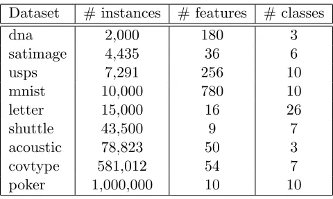
In this section, we evaluate the multi-class versions of FOGD and NOGD algorithms on 9 real-world datasets for multi-class classification tasks from the LIBSVM website. Table 6 summarizes the details of these datasets.
We adopt the same set of compared algorithms and similar parameter settings in
multi-class task as that of binary case. Larger the budget size parameterB is used for multiclass
Dataset # instances # features # classes
dna 2,000 180 3
satimage 4,435 36 6
usps 7,291 256 10
mnist 10,000 780 10
letter 15,000 16 26
shuttle 43,500 9 7
acoustic 78,823 50 3
covtype 581,012 54 7
poker 1,000,000 10 10
Table 6: Details of Multi-class Classification Datasets.
7.3.2 Performance Evaluation Results
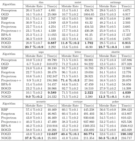
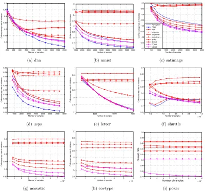
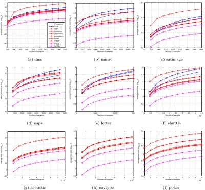
Table 7 summarizes the average performance evaluation results for the compared algorithms on multi-class classification task. To further inspect more details of online multi-class clas-sification performance, Figure 1 and Figure 2 also show the online performance convergence of all the compared algorithms in the entire online learning process. From these results, we can draw some observations as follows.
First of all, similar to the binary case, budget online kernel learning algorithms are much more efficient than the regular online kernel learning algorithms without budget, which is more obvious for larger scale datasets. For the three largest datasets (acoustic,covtypeand
poker), some of which consists of nearly one million instances, we have to exclude the non-budget online learning algorithms due to their extremely expensive costs in both time and memory. This again demonstrates the importance of exploring budget online kernel learning algorithms. Among the two non-budget online kernel learning algorithms, we found that OGD often achieves the highest accuracy, which is much better than Perceptron. However, its high-accuracy performance is paid by spending significantly higher computational time cost in comparison to the Perceptron algorithm. This is because OGD performs much more aggressive updates than Perceptron in the online learning process, which thus results in a significantly larger number of support vectors.
Second, when comparing the performance of different existing budget online kernel learn-ing algorithms, it is clear to observe that the algorithms based on support vector projection strategy (projectron and projectron++) achieve significantly higher accuracy than the algo-rithms using simple support vector removal strategy. However, the gain of accuracy is paid by the sacrifice of efficiency, as shown by the time cost results in the table. Furthermore, one might be surprised to observe that BPA-S, which is relatively efficient in binary case, is extremely slow in multi-class case. This is due to the different updating approach of BPA-S for multi-class classification. In particular, for other budget multi-class algorithms, their time complexity of each prediction is O(2B), i.e., only 2 out of the m classes (y and s) are updated when adding a new support vector. By contrast, during the update of BPA-S at each iteration, every class has to be updated, leading to the overall time complexity of
Algorithm dna mnist satimage
Mistake Rate Time(s) Mistake Rate Time(s) Mistake Rate Time(s)
Perceptron 20.4 %±0.7 4.891 15.4 %±0.1 456.76 29.6 %±0.5 4.675
OGD 16.1 %±0.4 25.068 10.7 %±0.2 1004.65 23.6 %±0.3 6.917
RBP 31.1 %±1.4 2.707 43.4 %±0.5 59.98 49.3 %±0.8 2.409
Forgetron 30.9 %±2.1 2.949 43.9 %±0.6 64.32 48.2 %±1.4 2.503
Projectron 22.7 %±4.4 4.254 17.7 %±0.1 434.53 29.6 %±0.5 3.685
Projectron++ 23.1 %±6.1 4.330 17.7 %±0.3 430.38 25.9 %±0.4 3.771
BPA-S 25.3 %±1.2 11.055 32.4 %±1.2 91.25 27.9 %±0.3 17.337
BOGD 36.3 %±0.9 3.103 42.5 %±0.4 62.51 48.2 %±0.6 2.670
FOGD 20.8 %±0.7 0.887 11.8 %±0.2 1.792 29.5 %±0.4 0.915
NOGD 20.7 %±0.9 2.292 15.6 %±0.6 46.90 23.7 %±0.3 1.869
Algorithm usps letter shuttle
Mistake Rate Time(s) Mistake Rate Time(s) Mistake Rate Time(s)
Perceptron 10.0 %±0.2 89.790 71.5 %±0.5 80.901 15.2 %±0.3 137.886
OGD 6.7 %±0.2 310.072 71.2 %±0.3 94.222 12.3 %±0.1 377.328
RBP 24.0 %±0.4 30.180 91.7 %±0.2 18.783 29.3 %±0.5 12.989
Forgetron 22.7 %±0.5 30.478 96.1 %±0.1 19.034 34.1 %±0.4 12.776
Projectron 10.6 %±0.1 192.347 71.5 %±0.5 26.921 15.3 %±0.3 20.034
Projectron++ 9.9 %±0.2 194.366 71.4 %±0.3 27.584 16.8 %±0.5 20.879
BPA-S 15.4 %±0.6 54.457 84.6 %±0.5 47.459 14.1 %±0.2 58.856
BOGD 23.2 %±0.4 30.966 92.7 %±0.2 18.510 27.9 %±0.2 14.399
FOGD 10.1 %±0.2 9.589 71.5 %±0.6 2.322 15.6 %±0.5 4.039
NOGD 9.0 %±0.2 24.332 71.5 %±0.2 3.380 12.3 %±0.1 8.484
Algorithm acoustic covtype poker
Mistake Rate Time(s) Mistake Rate Time(s) Mistake Rate Time(s)
RBP 57.4 %±0.2 40.469 60.1 %±0.1 445.238 56.6 %±0.0 398.423
Forgetron 61.2 %±0.4 46.865 60.4 %±0.4 491.403 56.5 %±0.0 413.807
Projectron 43.0 %±0.1 46.469 41.1 %±0.2 930.646 54.5 %±0.1 810.421
Projectron++ 40.3 %±0.1 47.400 38.3 %±0.2 937.860 53.2 %±0.1 825.526
BPA-S 46.2 %±0.3 210.916 45.2 %±0.2 1569.255 54.7 %±0.4 2566.812
BOGD 58.0 %±0.1 40.266 57.4 %±0.0 456.692 53.2 %±0.0 465.020
FOGD 43.0 %±0.2 12.637 40.4 %±0.1 80.774 52.6 %±0.1 190.102
NOGD 37.8 %±0.1 25.883 41.0 %±0.6 211.354 50.3 %±0.2 216.717