Learning Graphical Models With Hubs

Learning Graphical Models With Hubs

Kean Ming Tan [email protected]

Department of Biostatistics University of Washington Seattle WA, 98195

Palma London [email protected]

Karthik Mohan [email protected]

Department of Electrical Engineering University of Washington

Seattle WA, 98195

Su-In Lee [email protected]

Department of Computer Science and Engineering, Genome Sciences University of Washington

Seattle WA, 98195

Maryam Fazel [email protected]

Department of Electrical Engineering University of Washington

Seattle WA, 98195

Daniela Witten [email protected]

Department of Biostatistics University of Washington Seattle, WA 98195

Editor:Xiaotong Shen

Abstract

We consider the problem of learning a high-dimensional graphical model in which there are a fewhub nodes that aredensely-connected to many other nodes. Many authors have studied the use of an `1 penalty in order to learn a sparse graph in the high-dimensional setting. However, the `1 penalty implicitly assumes that each edge is equally likely and independent of all other edges. We propose a general framework to accommodate more realistic networks with hub nodes, using a convex formulation that involves a row-column overlap norm penalty. We apply this general framework to three widely-used probabilistic graphical models: the Gaussian graphical model, the covariance graph model, and the binary Ising model. An alternating direction method of multipliers algorithm is used to solve the corresponding convex optimization problems. On synthetic data, we demonstrate that our proposed framework outperforms competitors that do not explicitly model hub nodes. We illustrate our proposal on a webpage data set and a gene expression data set.

1. Introduction

Graphical models are used to model a wide variety of systems, such as gene regulatory networks and social interaction networks. A graph consists of a set of p nodes, each rep-resenting a variable, and a set of edges between pairs of nodes. The presence of an edge between two nodes indicates a relationship between the two variables. In this manuscript, we consider two types of graphs: conditional independence graphs and marginal indepen-dence graphs. In a conditional indepenindepen-dence graph, an edge connects a pair of variables if and only if they are conditionally dependent—dependent conditional upon the other vari-ables. In a marginal independence graph, two nodes are joined by an edge if and only if they are marginally dependent—dependent without conditioning on the other variables.

In recent years, many authors have studied the problem of learning a graphical model in the high-dimensional setting, in which the number of variables pis larger than the number of observations n. Let X be a n×p matrix, with rows x1, . . . ,xn. Throughout the rest of

the text, we will focus on three specific types of graphical models:

1. AGaussian graphical model, wherex1, . . . ,xn

i.i.d.

∼ N(0,Σ). In this setting, (Σ−1₎

jj0 =

0 for somej6=j0if and only if thejth andj0th variables are conditionally independent (Mardia et al., 1979); therefore, the sparsity pattern ofΣ−1_{determines the conditional}

independence graph.

2. A Gaussian covariance graph model, where x1, . . . ,xn

i.i.d.

∼ N(0,Σ). Then Σjj0 = 0

for some j 6=j0 if and only if the jth andj0th variables are marginally independent. Therefore, the sparsity pattern of Σdetermines the marginal independence graph.

3. A binary Ising graphical model, wherex1, . . . ,xn are i.i.d. with density function

p(x,Θ) = 1

Z(Θ)exp 



p

X

j=1

θjjxj+

X

1≤j<j0_≤p

θjj0x_jx_j0



,

where Θ is a p×p symmetric matrix, and Z(Θ) is the partition function, which ensures that the density sums to one. Here, xis a binary vector, and θjj0 = 0 if and

only if thejth andj0th variables are conditionally independent. The sparsity pattern of Θdetermines the conditional independence graph.

To construct an interpretable graph when p > n, many authors have proposed applying an `1 penalty to the parameter encoding each edge, in order to encourage sparsity. For

instance, such an approach is taken by Yuan and Lin (2007a), Friedman et al. (2007), Rothman et al. (2008), and Yuan (2008) in the Gaussian graphical model; El Karoui (2008), Bickel and Levina (2008), Rothman et al. (2009), Bien and Tibshirani (2011), Cai and Liu (2011), and Xue et al. (2012) in the covariance graph model; and Lee et al. (2007), H¨ofling and Tibshirani (2009), and Ravikumar et al. (2010) in the binary model.

However, applying an `1 penalty to each edge can be interpreted as placing an

of edges (Erd˝os and R´enyi, 1959). This is unrealistic in many real-world networks, in which we believe that certain nodes (which, unfortunately, are not known a priori) have a lot more edges than other nodes. An example is the network of webpages in the World Wide Web, where a relatively small number of webpages are connected to many other webpages (Barab´asi and Albert, 1999). A number of authors have shown that real-world networks

are scale-free, in the sense that the number of edges for each node follows a power-law

distribution; examples include gene-regulatory networks, social networks, and networks of collaborations among scientists (among others, Barab´asi and Albert, 1999; Barab´asi, 2009; Liljeros et al., 2001; Jeong et al., 2001; Newman, 2000; Li et al., 2005). More recently, Hao et al. (2012) have shown that certain genes, referred to assuper hubs, regulate hundreds of downstream genes in a gene regulatory network, resulting in far denser connections than are typically seen in a scale-free network.

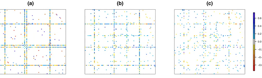
In this paper, we refer to very densely-connected nodes, such as the “super hubs” con-sidered in Hao et al. (2012), as hubs. When we refer to hubs, we have in mind nodes that are connected to a very substantial number of other nodes in the network—and in partic-ular, we are referring to nodes that are much more densely-connected than even the most highly-connected node in a scale-free network. An example of a network containing hub nodes is shown in Figure 1.

Here we propose a convex penalty function for estimating graphs containing hubs. Our formulation simultaneously identifies the hubs and estimates the entire graph. The penalty function yields a convex optimization problem when combined with a convex loss function. We consider the application of this hub penalty function in modeling Gaussian graphical models, covariance graph models, and binary Ising models. Our formulation does not require that we knowa priori which nodes in the network are hubs.

In related work, several authors have proposed methods to estimate a scale-free Gaussian graphical model (Liu and Ihler, 2011; Defazio and Caetano, 2012). However, those methods do not model hub nodes—the most highly-connected nodes that arise in a scale-free network are far less connected than the hubs that we consider in our formulation. Under a different framework, some authors proposed a screening-based procedure to identify hub nodes in the context of Gaussian graphical models (Hero and Rajaratnam, 2012; Firouzi and Hero, 2013). Our proposal outperforms such approaches when hub nodes are present (see discussion in Section 3.5.4).

In Figure 1, the performance of our proposed approach is shown in a toy example in the context of a Gaussian graphical model. We see that when the true network contains hub nodes (Figure 1(a)), our proposed approach (Figure 1(b)) is much better able to recover the network than is the graphical lasso (Figure 1(c)), a well-studied approach that applies an `1 penalty to each edge in the graph (Friedman et al., 2007).

We present the hub penalty function in Section 2. We then apply it to the Gaussian graphical model, the covariance graph model, and the binary Ising model in Sections 3, 4, and 5, respectively. In Section 6, we apply our approach to a webpage data set and a gene expression data set. We close with a discussion in Section 7.

2. The General Formulation

(a) (b) (c)

−0.6 −0.4 −0.2 0.0 0.2 0.4 0.6

Figure 1: (a): Heatmap of the inverse covariance matrix in a toy example of a Gaussian graphical model with four hub nodes. White elements are zero and colored el-ements are non-zero in the inverse covariance matrix. Thus, colored elel-ements correspond to edges in the graph. (b): Estimate from the hub graphical lasso, proposed in this paper. (c): Graphical lasso estimate.

2.1 The Hub Penalty Function

Let X be a n×p data matrix, Θ a p×p symmetric matrix containing the parameters of interest, and `(X,Θ) a loss function (assumed to be convex in Θ). In order to obtain a sparse and interpretable graph estimate, many authors have considered the problem

minimize

Θ∈S {`(X,Θ) +λkΘ−diag(Θ)k1}, (1)

whereλis a non-negative tuning parameter, S is some set depending on the loss function,

and k · k1 is the sum of the absolute values of the matrix elements. For instance, in the

case of a Gaussian graphical model, we could take `(X,Θ) =−log detΘ+ trace(SΘ), the negative log-likelihood of the data, where Sis the empirical covariance matrix andS is the set of p×p positive definite matrices. The solution to (1) can then be interpreted as an estimate of the inverse covariance matrix. The `1 penalty in (1) encourages zeros in the

solution. But it typically does not yield an estimate that contains hubs.

In order to explicitly model hub nodes in a graph, we wish to replace the `1 penalty in

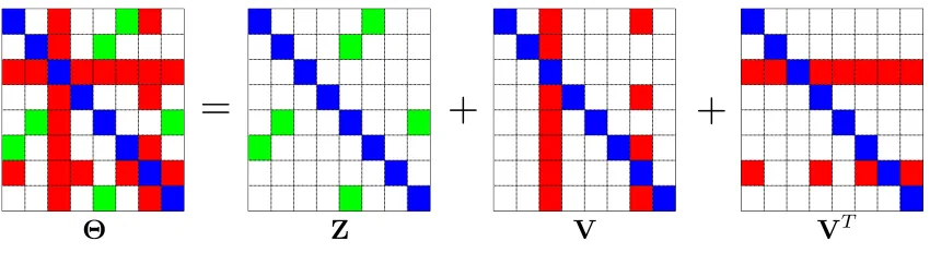
(1) with a convex penalty that encourages a solution that can be decomposed asZ+V+VT_,

whereZis a sparse symmetric matrix, andV is a matrix whose columns are either entirely zero or almost entirely non-zero (see Figure 2). The sparse elements of Zrepresent edges between non-hub nodes, and the non-zero columns of V correspond to hub nodes. We achieve this goal via thehub penalty function, which takes the form

P(Θ) = min V,Z: Θ=V+VT+Z

(

λ1kZ−diag(Z)k1+λ2kV−diag(V)k1+λ3

p

X

j=1

k(V−diag(V))jkq

)

. (2)

Hereλ1, λ2, andλ3 are nonnegative tuning parameters. Sparsity inZis encouraged via the `1 penalty on its off-diagonal elements, and is controlled by the value of λ1. The `1 and `1/`q norms on the columns of V induce group sparsity whenq = 2 (Yuan and Lin, 2007b;

=

+

+

⇥

Z

V

V

Figure 2: Decomposition of a symmetric matrixΘintoZ+V+VT_{, whereZis sparse, and}

most columns of V are entirely zero. Blue, white, green, and red elements are diagonal, zero, non-zero inZ, and non-zero due to two hubs in V, respectively.

each hub node’s connections to other nodes. The convex penalty (2) can be combined with

`(X,Θ) to yield the convex optimization problem

minimize Θ∈S,V,Z

(

`(X,Θ) +λ1kZ−diag(Z)k1+λ2kV−diag(V)k1

+λ3

p

X

j=1

k(V−diag(V))jkq

)

subject to Θ=V+VT +Z, (3)

where the setS depends on the loss function`(X,Θ).

Note that when λ2 → ∞ or λ3 → ∞, then (3) reduces to (1). In this paper, we take q = 2, which leads to estimation of a network containing dense hub nodes. Other values of q such asq =∞ are also possible (see, e.g., Mohan et al., 2014). We note that the hub penalty function is closely related to recent work on overlapping group lasso penalties in the context of learning multiple sparse precision matrices (Mohan et al., 2014).

2.2 Algorithm

In order to solve (3) with q = 2, we use an alternating direction method of multipliers

(ADMM) algorithm (see, e.g., Eckstein and Bertsekas, 1992; Boyd et al., 2010; Eckstein, 2012). ADMM is an attractive algorithm for this problem, as it allows us to decouple some of the terms in (3) that are difficult to optimize jointly. In order to develop an ADMM algorithm for (3) with guaranteed convergence, we reformulate it as a consensus problem, as in Ma et al. (2013). The convergence of the algorithm to the optimal solution follows from classical results (see, e.g., the review papers Boyd et al., 2010; Eckstein, 2012).

In greater detail, we let B= (Θ,V,Z), ˜B= ( ˜Θ,V˜,Z˜),

f(B) =`(X,Θ) +λ1kZ−diag(Z)k1+λ2kV−diag(V)k1+λ3

p

X

j=1

Algorithm 1 ADMM Algorithm for Solving (3).

1. Initializethe parameters:

(a) primal variablesΘ,V,Z,Θ˜,V˜, and ˜Zto thep×pidentity matrix. (b) dual variablesW1,W2, andW3to thep×pzero matrix.

(c) constantsρ >0 andτ >0.

2. Iterate until the stopping criterion kΘt−Θt−1k2F

kΘt−1k2F

≤ τ is met, where Θt is the value of Θ obtained at thetth iteration:

(a) UpdateΘ,V,Z:

i. Θ= arg min Θ∈S

n

`(X,Θ) +ρ₂kΘ−Θ˜ +W1k2F

o

.

ii. Z=S( ˜Z−W3,λ_ρ1), diag(Z) = diag( ˜Z−W3). HereSdenotes the soft-thresholding operator, applied element-wise to a matrix: S(Aij, b) = sign(Aij) max(|Aij| −b,0). iii. C= ˜V−W2−diag( ˜V−W2).

iv. Vj= max1− λ3

ρkS(Cj,λ2/ρ)k2,0

·S(Cj, λ2/ρ) forj= 1, . . . , p.

v. diag(V) = diag( ˜V−W2). (b) Update ˜Θ,V˜,Z˜:

i. Γ= ρ₆

(Θ+W1)−(V+W2)−(V+W2)T _−(Z+W3)

.

ii. ˜Θ=Θ+W1−_ρ1Γ; iii. ˜V=1_ρ(Γ+ΓT) +V+W2; iv. ˜Z= 1_ρΓ+Z+W3.

(c) UpdateW1,W2,W3:

and

g( ˜B) = (

0 if ˜Θ= ˜V+ ˜VT _{+ ˜Z} ∞ otherwise.

Then, we can rewrite (3) as

minimize B,B˜

n

f(B) +g( ˜B)o subject to B= ˜B. (4)

The scaled augmented Lagrangian for (4) takes the form

L(B,B˜,W) =`(X,Θ) +λ1kZ−diag(Z)k1+λ2kV−diag(V)k1

+λ3

p

X

j=1

k(V−diag(V))jk2+g( ˜B) + ρ

2kB−B˜ +Wk

2

F,

where B and ˜B are the primal variables, and W = (W1,W2,W3) is the dual variable. Note that the scaled augmented Lagrangian can be derived from the usual Lagrangian by adding a quadratic term and completing the square (Boyd et al., 2010).

A general algorithm for solving (3) is provided in Algorithm 1. The derivation is in Appendix A. Note that only the update for Θ (Step 2(a)i) depends on the form of the convex loss function `(X,Θ). In the following sections, we consider special cases of (3) that lead to estimation of Gaussian graphical models, covariance graph models, and binary networks with hub nodes.

3. The Hub Graphical Lasso

Assume that x1, . . . ,xn i.∼i.d. N(0,Σ). The well-known graphical lasso problem (see, e.g.,

Friedman et al., 2007) takes the form of (1) with `(X,Θ) = −log detΘ+ trace(SΘ), and

S the empirical covariance matrix ofX:

minimize

Θ∈S







−log detΘ+ trace(SΘ) +λX

j6=j0

|Θjj0|







, (5)

whereS ={Θ:Θ0 and Θ=ΘT_{}. The solution to this optimization problem serves as}

an estimate forΣ−1_{. We now use the hub penalty function to extend the graphical lasso in}

order to accommodate hub nodes.

3.1 Formulation and Algorithm

We propose the hub graphical lasso (HGL) optimization problem, which takes the form

minimize

Θ∈S {−log detΘ+ trace(SΘ) + P(Θ)}. (6)

Again,S ={Θ:Θ0 and Θ=ΘT_{}. It encourages a solution that contains hub nodes, as}

well as edges that connect non-hubs (Figure 1). Problem (6) can be solved using Algorithm 1. The update for Θin Algorithm 1 (Step 2(a)i) can be derived by minimizing

−log detΘ+ trace(SΘ) +ρ

2kΘ−Θ˜ +W1k

2

with respect toΘ(note that the constraintΘ∈ S in (6) is treated as an implicit constraint, due to the domain of definition of the log det function). This can be shown to have the solution

Θ= 1 2U

D+ r

D2₊4 ρI

UT,

whereUDUT denotes the eigen-decomposition of ˜Θ−W1−1_ρS.

The complexity of the ADMM algorithm for HGL is O(p3) per iteration; this is the complexity of the eigen-decomposition for updating Θ. We now briefly compare the com-putational time for the ADMM algorithm for solving (6) to that of an interior point method (using the solver Sedumicalled from cvx). On a 1.86 GHz Intel Core 2 Duo machine, the interior point method takes ∼3 minutes, while ADMM takes only 1 second, on a data set with p = 30. We present a more extensive run time study for the ADMM algorithm for HGL in Appendix E.

3.2 Conditions for HGL Solution to be Block Diagonal

In order to reduce computations for solving the HGL problem, we now present a necessary condition and a sufficient condition for the HGL solution to be block diagonal, subject to some permutation of the rows and columns. The conditions depend only on the tuning parameters λ1, λ2, and λ3. These conditions build upon similar results in the context

of Gaussian graphical models from the recent literature (see, e.g., Witten et al., 2011; Mazumder and Hastie, 2012; Yang et al., 2012b; Danaher et al., 2014; Mohan et al., 2014). LetC1, C2, . . . , CK denote a partition of thep features.

Theorem 1 A sufficient condition for the HGL solution to be block diagonal with blocks

given by C1, C2, . . . , CK is that min

n

λ1,λ₂2

o

>|Sjj0|for all j∈C_k, j0 ∈C_k0, k6=k0.

Theorem 2 A necessary condition for the HGL solution to be block diagonal with blocks

given by C1, C2, . . . , CK is that min

n

λ1,λ2+₂λ3

o

>|Sjj0| for allj ∈C_k, j0 ∈C_k0, k6=k0.

Theorem 1 implies that one can screen the empirical covariance matrix S to check if the HGL solution is block diagonal (using standard algorithms for identifying the connected components of an undirected graph; see, e.g., Tarjan, 1972). Suppose that the HGL solution is block diagonal with K blocks, containing p1, . . . , pK features, and

PK

k=1pk = p. Then,

one can simply solve the HGL problem on the features within each block separately. Recall that the bottleneck of the HGL algorithm is the eigen-decomposition for updatingΘ. The block diagonal condition leads to massive computational speed-ups for implementing the HGL algorithm: instead of computing an eigen-decomposition for a p×p matrix in each iteration of the HGL algorithm, we compute the eigen-decomposition of K matrices of dimensions p1 ×p1, . . . , pK×pK. The computational complexity per-iteration is reduced

from O(p3) to PK

k=1O(p3k).

We illustrate the reduction in computational time due to these results in an example with

3.3 Some Properties of HGL

We now present several properties of the HGL optimization problem (6), which can be used to provide guidance on the suitable range for the tuning parametersλ1,λ2, andλ3. In what

follows,Z∗ and V∗ denote the optimal solutions for Zand V in (6). Let 1_s +1_q = 1 (recall thatq appears in Equation 2).

Lemma 3 A sufficient condition for Z∗ _{to be a diagonal matrix is that λ}

1 > λ2+₂λ3. Lemma 4 A sufficient condition forV∗ to be a diagonal matrix is thatλ1< λ₂2+_2(p−λ₁₎31/s. Corollary 5 A necessary condition for both V∗ andZ∗ to be non-diagonal matrices is that

λ2

2 +

λ3

2(p−1)1/s ≤λ1 ≤

λ2+λ3

2 .

Furthermore, (6) reduces to the graphical lasso problem (5) under a simple condition.

Lemma 6 If q = 1, then (6) reduces to (5) with tuning parameter minnλ1,λ2+₂λ3

o

.

Note also that when λ2 → ∞ or λ3 → ∞, (6) reduces to (5) with tuning parameter λ1.

However, throughout the rest of this paper, we assume thatq= 2, andλ2 andλ3 are finite.

The solution ˆΘof (6) is unique, since (6) is a strictly convex problem. We now consider the question of whether the decomposition ˆΘ = ˆV + ˆVT _{+ ˆZ is unique. We see that}

the decomposition is unique in a certain regime of the tuning parameters. For instance, according to Lemma 3, when λ1 > λ2+₂λ3, ˆZis a diagonal matrix and hence ˆV is unique.

Similarly, according to Lemma 4, when λ1 < λ₂2 + _2(p−λ₁₎31/s, ˆV is a diagonal matrix and

hence ˆZis unique. Studying more general conditions on S and onλ1,λ2, andλ3 such that

the decomposition is guaranteed to be unique is a challenging problem and is outside of the scope of this paper.

3.4 Tuning Parameter Selection

In this section, we propose a Bayesian information criterion (BIC)-type quantity for tun-ing parameter selection in (6). Recall from Section 2 that the hub penalty function (2) decomposes the parameter of interest into the sum of three matrices, Θ = Z+V+VT, and places an `1 penalty on Z, and an `1/`2 penalty onV.

For the graphical lasso problem in (5), many authors have proposed to select the tuning parameterλsuch that ˆΘminimizes the following quantity:

−n·log det( ˆΘ) +n·trace(SΘˆ) + log(n)· |Θˆ|,

where |Θˆ|is the cardinality of ˆΘ, that is, the number of unique non-zeros in ˆΘ(see, e.g., Yuan and Lin, 2007a).1

1. The term log(n)· |Θ|ˆ is motivated by the fact that the degrees of freedom for an estimate involving the

Using a similar idea, we propose the following BIC-type quantity for selecting the set of tuning parameters (λ1, λ2, λ3) for (6):

BIC( ˆΘ,Vˆ,Zˆ) =−n·log det( ˆΘ) +n·trace(SΘˆ) + log(n)· |Zˆ|+ log(n)·ν+c·[|Vˆ| −ν],

whereνis the number of estimated hub nodes, that is,ν =Pp

j=11{k_Vˆ_jk0>0},cis a constant

between zero and one, and |Zˆ| and |Vˆ| are the cardinalities (the number of unique non-zeros) of ˆZ and ˆV, respectively.2 _{We select the set of tuning parameters (λ}

1, λ2, λ3) for

which the quantity BIC( ˆΘ,Vˆ,Zˆ) is minimized. Note that when the constant c is small, BIC( ˆΘ,Vˆ,Zˆ) will favor more hub nodes in ˆV. In this manuscript, we take c= 0.2.

3.5 Simulation Study

In this section, we compare HGL to two sets of proposals: proposals that learn an Erd˝os-R´enyi Gaussian graphical model, and proposals that learn a Gaussian graphical model in which some nodes are highly-connected.

3.5.1 Notation and Measures of Performance

We start by defining some notation. Let ˆΘ be the estimate of Θ = Σ−1 _{from a given}

proposal, and let ˆΘj be itsjth column. LetHdenote the set of indices of the hub nodes in

Θ(that is, this is the set of true hub nodes in the graph), and let|H|denote the cardinality of the set. In addition, let ˆH_r be the set of estimated hub nodes: the set of nodes in ˆΘ

that are among the |H|most highly-connected nodes, and that have at least r edges. The values chosen for |H| and r depend on the simulation set-up, and will be specified in each simulation study.

We now define several measures of performance that will be used to evaluate the various methods.

• Number of correctly estimated edges: P

j<j0

1_{|Θˆ

jj0|>10−5 and|Θjj0|6=0}

.

• Proportion of correctly estimated hub edges:

P

j∈H,j0_6=j

1_{|Θˆ

jj0|>10−5 and|Θjj0|6=0}

P

j∈H,j0_6=j

1{|Θjj0|6=0}

.

• Proportion of correctly estimated hub nodes:|Hˆr∩H|

|H| .

• Sum of squared errors: P

j<j0

ˆ

Θjj0−Θ_jj0

2 .

2. The term log(n)· |Z|ˆ is motivated by the degrees of freedom from the`1penalty, and the term log(n)·

3.5.2 Data Generation

We consider three set-ups for generating ap×p adjacency matrix A.

I - Network with hub nodes: for alli < j, we setAij = 1 with probability 0.02, and zero

otherwise. We then set Aji equal to Aij. Next, we randomly select |H| hub nodes

and set the elements of the corresponding rows and columns ofA to equal one with probability 0.7 and zero otherwise.

II - Network with two connected components and hub nodes: the adjacency matrix is

generated asA=

A1 0

0 A2

, with A1 and A2 as in Set-up I, each with |H|/2 hub

nodes.

III - Scale-free network:3 _{the probability that a given node has k edges is proportional}

to k−α. Barab´asi and Albert (1999) observed that many real-world networks have

α ∈ [2.1,4]; we took α = 2.5. Note that there is no natural notion of hub nodes in a scale-free network. While some nodes in a scale-free network have more edges than one would expect in an Erd˝os-R´enyi graph, there is no clear distinction between “hub” and “non-hub” nodes, unlike in Set-ups I and II. In our simulation settings, we consider any node that is connected to more than 5% of all other nodes to be a hub node.4

We then use the adjacency matrix Ato create a matrixE, as

Eij i.∼i.d.

(

0 ifAij = 0

Unif([−0.75,−0.25]∪[0.25,0.75]) otherwise,

and set ¯E = 1₂(E+ET_{). Given the matrix ¯E, we set Σ}−1 _{equal to ¯E+ (0.1−Λ}

min( ¯E))I,

where Λmin( ¯E) is the smallest eigenvalue of ¯E. We generate the data matrixXaccording to x1, . . . ,xn

i.i.d.

∼ N(0,Σ). Then, variables are standardized to have standard deviation one.

3.5.3 Comparison to Graphical Lasso and Neighbourhood Selection

In this subsection, we compare the performance of HGL to two proposals that learn a sparse Gaussian graphical model.

• The graphical lasso (5), implemented using the Rpackageglasso.

• The neighborhood selection approach of Meinshausen and B¨uhlmann (2006), imple-mented using theRpackageglasso. This approach involves performingp `1-penalized

regression problems, each of which involves regressing one feature onto the others.

3. Recall that our proposal is not intended for estimating a scale-free network.

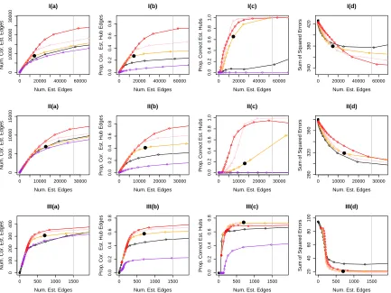
We consider the three simulation set-ups described in the previous section withn= 1000,

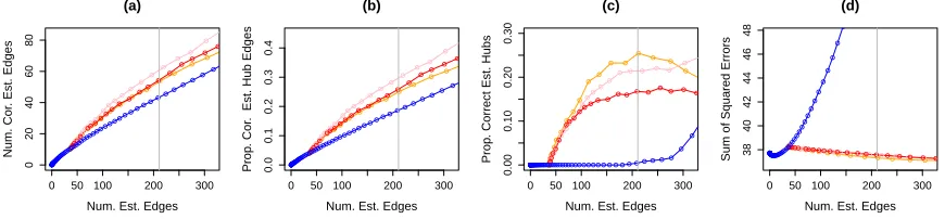
p= 1500, and|H|= 30 hub nodes in Set-ups I and II. Figure 3 displays the results, averaged over 100 simulated data sets. Note that the sum of squared errors is not computed for Meinshausen and B¨uhlmann (2006), since it does not directly yield an estimate ofΘ=Σ−1_.

HGL has three tuning parameters. To obtain the curves shown in Figure 3, we fixed

λ1 = 0.4, considered three values of λ3 (each shown in a different color in Figure 3), and

used a fine grid of values ofλ2. The solid black circle in Figure 3 corresponds to the set of

tuning parameters (λ1, λ2, λ3) for which the BIC as defined in Section 3.4 is minimized. The

graphical lasso and Meinshausen and B¨uhlmann (2006) each involves one tuning parameter; we applied them using a fine grid of the tuning parameter to obtain the curves shown in Figure 3.

Results for Set-up I are displayed in Figures 3-I(a) through 3-I(d), where we calculate the proportion of correctly estimated hub nodes as defined in Section 3.5.1 with r = 300. Since this simulation set-up exactly matches the assumptions of HGL, it is not surprising that HGL outperforms the other methods. In particular, HGL is able to identify most of the hub nodes when the number of estimated edges is approximately equal to the true number of edges. We see similar results for Set-up II in Figures 3-II(a) through 3-II(d), where the proportion of correctly estimated hub nodes is as defined in Section 3.5.1 withr = 150.

In Set-up III, recall that we define a node that is connected to at least 5% of all nodes to be a hub. The proportion of correctly estimated hub nodes is then as defined in Section 3.5.1 with r = 0.05×p. The results are presented in Figures 3-III(a) through 3-III(d). In this set-up, only approximately three of the nodes (on average) have more than 50 edges, and the hub nodes are not as highly-connected as in Set-up I or Set-up II. Nonetheless, HGL outperforms the graphical lasso and Meinshausen and B¨uhlmann (2006).

Finally, we see from Figure 3 that the set of tuning parameters (λ1, λ2, λ3) selected using

BIC performs reasonably well. In particular, the graphical lasso solution always has BIC larger than HGL, and hence, is not selected.

3.5.4 Comparison to Additional Proposals

In this subsection, we compare the performance of HGL to three additional proposals:

• The partial correlation screening procedure of Hero and Rajaratnam (2012). The elements of the partial correlation matrix (computed using a pseudo-inverse when

p > n) are thresholded based on their absolute value, and a hub node is declared if the number of nonzero elements in the corresponding column of the thresholded partial correlation matrix is sufficiently large. Note that the purpose of Hero and Rajaratnam (2012) is to screen for hub nodes, rather than to estimate the individual edges in the network.

• The scale-free network estimation procedure of Liu and Ihler (2011). This is the solution to the non-convex optimization problem

minimize Θ∈S







−log detΘ+ trace(SΘ) +α

p

X

j=1

log(kθ\jk1+j) + p

X

j=1

βj|θjj|







0 20000 40000 60000 0 10000 20000 30000 I(a)

Num. Est. Edges

Num. Cor

. Est. Edges

● ● ● ● ● ● ● ● ● ● ● ● ● ● ● ● ● ● ● ● ● ● ● ● ● ● ● ● ● ● ● ● ● ● ● ● ● ● ● ● ● ● ● ● ● ● ● ● ● ● ● ● ● ● ● ● ● ● ● ● ● ● ● ● ● ● ● ● ● ● ● ● ● ● ● ● ● ● ● ● ● ● ● ● ● ● ● ● ● ● ● ● ● ● ● ● ● ● ● ● ● ● ● ● ● ● ● ● ● ● ● ● ● ● ● ● ● ● ● ● ● ● ● ● ● ● ● ● ● ● ● ● ● ● ● ● ● ● ● ● ● ● ● ● ● ● ● ● ● ● ●

0 20000 40000 60000

0.0 0.2 0.4 0.6 0.8 I(b)

Num. Est. Edges

Prop

. Cor

. Est. Hub Edges

● ● ● ● ● ● ● ● ● ● ● ● ● ● ● ● ● ● ● ● ● ● ● ● ● ● ● ● ● ● ● ● ● ● ● ● ● ● ● ● ● ● ● ● ● ● ● ● ● ● ● ● ● ● ● ● ● ● ● ● ● ● ● ● ● ● ● ● ● ● ● ● ● ● ● ● ● ● ● ● ● ● ● ● ● ● ● ● ● ● ● ● ● ● ● ● ● ● ● ● ● ● ● ● ● ● ● ● ● ● ● ● ● ● ● ● ● ● ● ● ● ● ● ● ● ● ● ● ● ● ● ● ● ● ● ● ● ● ● ● ● ● ● ● ● ● ● ● ●

0 20000 40000 60000

0.0 0.2 0.4 0.6 0.8 1.0 I(c)

Num. Est. Edges

Prop

. Correct Est. Hubs

● ● ● ● ● ● ● ● ● ● ● ● ● ● ● ● ● ● ● ● ● ● ● ● ● ● ● ● ● ● ● ● ● ● ● ● ● ● ● ● ● ● ● ● ● ● ● ● ● ● ● ● ● ● ● ● ● ● ● ● ● ● ● ● ● ● ● ● ● ● ● ● ● ● ● ● ● ● ● ● ● ● ● ● ● ● ● ● ● ● ● ● ● ● ● ● ● ● ● ● ● ● ● ● ● ● ● ● ● ● ● ● ● ● ●●●●●●●●●●●●●●●●● ● ● ● ● ● ● ● ● ● ● ● ● ● ●

0 20000 40000 60000

340

380

420

I(d)

Num. Est. Edges

Sum of Squared Errors

● ● ● ● ● ● ● ● ● ● ● ● ● ● ● ● ● ● ● ● ● ● ● ● ● ● ● ● ● ● ● ● ● ● ● ● ● ● ● ● ● ● ● ● ● ● ● ● ● ● ● ● ● ● ● ● ● ● ● ● ● ● ● ● ● ● ● ● ● ● ● ● ● ● ● ● ● ● ● ● ● ● ● ● ● ● ● ● ● ● ● ● ● ● ● ● ● ● ● ● ● ● ● ● ● ● ● ● ● ● ● ● ● ●

0 10000 20000 30000

0

5000

10000

15000

II(a)

Num. Est. Edges

Num. Cor

. Est. Edges

● ● ● ● ● ● ● ● ● ● ● ● ● ● ● ● ● ● ● ● ● ● ● ● ● ● ● ● ● ● ● ● ● ● ● ● ● ● ● ● ● ● ● ● ● ● ● ● ● ● ● ● ● ● ● ● ● ● ● ● ● ● ● ● ● ● ● ● ● ● ● ● ● ● ● ● ● ● ● ● ● ● ● ● ● ● ● ● ● ● ● ● ● ● ● ● ● ● ● ● ● ● ● ● ● ● ● ● ● ● ● ● ● ● ● ● ● ● ● ● ● ● ● ● ● ● ● ● ● ● ● ● ● ● ● ● ● ● ● ● ● ● ● ● ● ●

0 10000 20000 30000

0.0 0.2 0.4 0.6 0.8 II(b)

Num. Est. Edges

Prop

. Cor

. Est. Hub Edges

● ● ● ● ● ● ● ● ● ● ● ● ● ● ● ● ● ● ● ● ● ● ● ● ● ● ● ● ● ● ● ● ● ● ● ● ● ● ● ● ● ● ● ● ● ● ● ● ● ● ● ● ● ● ● ● ● ● ● ● ● ● ● ● ● ● ● ● ● ● ● ● ● ● ● ● ● ● ● ● ● ● ● ● ● ● ● ● ● ● ● ● ● ● ● ● ● ● ● ● ● ● ● ● ● ● ● ● ● ● ● ● ● ● ● ● ● ● ● ● ● ● ● ● ● ● ● ● ● ● ● ● ● ● ● ● ● ● ● ● ● ● ● ●

0 10000 20000 30000

0.0 0.2 0.4 0.6 0.8 1.0 II(c)

Num. Est. Edges

Prop

. Correct Est. Hubs

● ● ● ● ● ● ● ● ● ● ● ● ● ● ● ● ● ● ● ● ● ● ● ● ● ● ● ● ● ● ● ● ● ● ● ● ● ● ● ● ● ● ● ● ● ● ● ● ● ● ● ● ● ● ● ● ● ● ● ● ● ● ● ● ● ● ● ● ● ● ● ● ● ● ● ● ● ● ● ● ● ● ● ● ● ● ● ● ● ● ● ● ● ● ● ● ● ● ● ● ● ● ● ● ● ● ● ● ● ● ● ● ●●●●●●●●●●●●●●●●●●● ● ● ● ● ● ● ● ● ● ●

0 10000 20000 30000

280

320

360

II(d)

Num. Est. Edges

Sum of Squared Errors

● ● ● ● ● ● ● ● ● ● ● ● ● ● ● ● ● ● ● ● ● ● ● ● ● ● ● ● ● ● ● ● ● ● ● ● ● ● ● ● ● ● ● ● ● ● ● ● ● ● ● ● ● ● ● ● ● ● ● ● ● ● ● ● ● ● ● ● ● ● ● ● ● ● ● ● ● ● ● ● ● ● ● ● ● ● ● ● ● ● ● ● ● ● ● ● ● ● ● ● ● ● ● ● ● ● ● ● ● ● ●

0 500 1000 1500

0 100 200 300 400 III(a)

Num. Est. Edges

Num. Cor

. Est. Edges

● ● ● ● ● ● ● ● ● ● ● ● ● ● ● ● ● ● ● ● ● ● ● ● ● ● ● ● ● ● ● ● ● ● ● ● ● ● ● ● ● ● ● ● ● ● ● ● ● ● ● ● ● ● ● ● ● ● ● ● ● ● ● ● ● ● ● ● ● ● ● ● ● ● ● ● ● ● ● ● ● ● ● ● ● ● ● ● ● ● ● ● ● ● ● ● ● ● ● ● ● ● ● ● ● ● ● ● ● ● ● ● ● ● ● ● ● ● ● ● ● ● ● ● ● ● ● ● ● ● ● ● ● ●

0 500 1000 1500

0.0 0.2 0.4 0.6 0.8 III(b)

Num. Est. Edges

Prop

. Cor

. Est. Hub Edges

● ● ● ● ● ● ● ● ● ● ● ● ● ● ● ● ● ● ● ● ● ● ● ● ● ● ● ● ● ● ● ● ● ● ● ● ● ● ● ● ● ● ● ● ● ● ● ● ● ● ● ● ● ● ● ● ● ● ● ● ● ● ● ● ● ● ● ● ● ● ● ● ● ● ● ● ● ● ● ● ● ● ● ● ● ● ● ● ● ● ● ● ● ● ● ● ● ● ● ● ● ● ● ● ● ● ● ● ● ● ● ● ● ● ● ● ● ● ● ● ● ● ● ● ● ● ● ● ● ● ● ●

0 500 1000 1500

0.0 0.2 0.4 0.6 0.8 III(c)

Num. Est. Edges

Prop

. Correct Est. Hubs

● ● ● ● ● ● ● ● ● ● ● ● ● ● ● ● ● ● ● ● ● ● ● ● ● ● ● ● ● ● ● ● ● ● ● ● ● ● ● ● ● ● ● ● ● ● ● ● ● ● ● ● ● ● ● ● ● ● ● ● ● ● ● ● ● ● ● ● ● ● ● ● ● ● ● ● ● ● ● ● ● ● ● ● ● ● ● ● ● ● ● ● ● ● ● ● ● ● ● ● ● ● ● ● ● ● ● ● ● ● ● ● ● ● ● ● ● ● ● ● ● ● ● ● ● ● ● ● ● ● ● ●

0 500 1000 1500

20 40 60 80 100 III(d)

Num. Est. Edges

Sum of Squared Errors

● ● ● ● ● ● ● ● ● ● ● ● ● ● ● ● ● ● ● ● ● ● ● ● ● ● ● ● ● ● ● ● ● ● ● ● ● ● ● ● ● ● ● ● ● ● ● ● ● ● ● ● ● ● ● ● ● ● ● ● ● ● ● ● ● ● ● ● ● ● ● ● ● ● ● ● ● ● ● ● ● ● ● ● ● ● ● ● ● ● ● ● ● ● ● ● ● ● ● ● ● ● ● ● ●

Figure 3: Simulation for Gaussian graphical model. Row I: Results for Set-up I. Row II: Results for Set-up II. Row III: Results for Set-up III. The results are forn= 1000 andp= 1500. In each panel, the x-axis displays the number of estimated edges, and the vertical gray line is the number of edges in the true network. They-axes are as follows: Column (a): Number of correctly estimated edges; Column (b): Proportion of correctly estimated hub edges; Column (c): Proportion of correctly estimated hub nodes; Column (d): Sum of squared errors. The black solid circles are the results for HGL based on tuning parameters selected using the BIC-type criterion defined in Section 3.4. Colored lines correspond to the graphical lasso (Friedman et al., 2007) ( ); HGL withλ3 = 0.5 ( ),λ3 = 1 ( ), andλ3 = 2

where θ\j ={θjj0|j0 6=j}, and _j, β_j, and α are tuning parameters. Here,S ={Θ: Θ0 and Θ=ΘT_}.

• Sparse partial correlation estimation procedure of Peng et al. (2009), implemented using the R package space. This is an extension of the neighborhood selection ap-proach of Meinshausen and B¨uhlmann (2006) that combinesp `1-penalized regression

problems in order to obtain a symmetric estimator. The authors claimed that the proposal performs well in estimating a scale-free network.

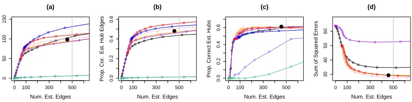
We generated data under Set-ups I and III (described in Section 3.5.2) with n = 250 and p= 500,5 _{and with |H|= 10 for Set-up I. The results, averaged over 100 data sets, are}

displayed in Figures 4 and 5.

To obtain Figures 4 and 5, we applied Liu and Ihler (2011) using a fine grid of αvalues, and using the choices forβj and j specified by the authors: βj = 2α/j, wherej is a small

constant specified in Liu and Ihler (2011). There are two tuning parameters in Hero and Rajaratnam (2012): (1) ρ, the value used to threshold the partial correlation matrix, and (2)d, the number of non-zero elements required for a column of the thresholded matrix to be declared a hub node. We used d={10,20} in Figures 4 and 5, and used a fine grid of values forρ. Note that the value ofd has no effect on the results for Figures 4(a)-(b) and Figures 5(a)-(b), and that larger values ofdtend to yield worse results in Figures 4(c) and 5(c). For Peng et al. (2009), we used a fine grid of tuning parameter values to obtain the curves shown in Figures 4 and 5. The sum of squared errors was not reported for Peng et al. (2009) and Hero and Rajaratnam (2012) since they do not directly yield an estimate of the precision matrix. As a baseline reference, the graphical lasso is included in the comparison. We see from Figure 4 that HGL outperforms the competitors when the underlying network contains hub nodes. It is not surprising that Liu and Ihler (2011) yields better results than the graphical lasso, since the former approach is implemented via an iterative procedure: in each iteration, the graphical lasso is performed with an updated tuning parameter based on the estimate obtained in the previous iteration. Hero and Rajaratnam (2012) has the worst results in Figures 4(a)-(b); this is not surprising, since the purpose of Hero and Rajaratnam (2012) is to screen for hub nodes, rather than to estimate the individual edges in the network.

From Figure 5, we see that the performance of HGL is comparable to that of Liu and Ihler (2011) and Peng et al. (2009) under the assumption of a scale-free network; note that this is the precise setting for which Liu and Ihler (2011)’s proposal is intended, and Peng et al. (2009) reported that their proposal performs well in this setting. In contrast, HGL is not intended for the scale-free network setting (as mentioned in the Introduction, it is intended for a setting with hub nodes). Again, Liu and Ihler (2011) and Peng et al. (2009) outperform the graphical lasso, and Hero and Rajaratnam (2012) has the worst results in Figures 5(a)-(b). Finally, we see from Figures 4 and 5 that the BIC-type criterion for HGL proposed in Section 3.4 yields good results.

0 2000 4000 6000 0 1000 2000 3000 (a)

Num. Est. Edges

Num. Cor

. Est. Edges

● ● ● ● ● ● ● ● ● ● ● ● ● ● ● ● ● ● ● ● ● ● ● ● ● ● ● ● ● ● ● ● ● ● ● ● ● ● ● ● ● ● ● ● ● ● ● ● ● ● ● ● ● ● ● ● ● ● ● ● ● ● ● ● ● ● ● ● ● ● ● ● ● ● ● ● ● ● ● ● ● ● ● ● ● ● ● ● ● ● ● ● ● ● ● ● ● ● ● ● ● ● ● ● ● ● ● ● ● ● ● ● ● ● ● ● ● ● ● ● ● ● ● ● ● ● ● ● ● ● ● ● ● ● ● ● ● ● ● ● ● ● ● ● ● ● ● ● ● ● ● ● ● ● ● ● ● ● ● ● ● ● ● ● ● ● ● ● ● ● ● ● ● ● ● ● ● ● ● ● ● ● ● ● ● ● ● ● ● ● ● ● ● ● ● ● ● ● ● ● ● ● ● ● ● ● ● ● ● ● ● ● ● ● ● ● ● ● ● ● ● ● ● ● ● ● ● ● ● ● ● ● ● ● ● ● ● ● ● ● ● ● ● ● ● ● ● ● ● ● ● ● ● ● ● ● ● ● ● ● ● ● ● ● ● ● ● ● ● ● ● ● ● ● ● ●

0 2000 4000 6000

0.0 0.2 0.4 0.6 0.8 (b)

Num. Est. Edges

Prop

. Cor

. Est. Hub Edges ●

● ● ● ● ● ● ● ● ● ● ● ● ● ● ● ● ● ● ● ● ● ● ● ● ● ● ● ● ● ● ● ● ● ● ● ● ● ● ● ● ● ● ● ● ● ● ● ● ● ● ● ● ● ● ● ● ● ● ● ● ● ● ● ● ● ● ● ● ● ● ● ● ● ● ● ● ● ● ● ● ● ● ● ● ● ● ● ● ● ● ● ● ● ● ● ● ● ● ● ● ● ● ● ● ● ● ● ● ● ● ● ● ● ● ● ● ● ● ● ● ● ● ● ● ● ● ● ● ● ● ● ● ● ● ● ● ● ● ● ● ● ● ● ● ● ● ● ● ● ● ● ● ● ● ● ● ● ● ● ● ● ● ● ● ● ● ● ● ● ● ● ● ● ● ● ● ● ● ● ● ● ● ● ● ● ● ● ● ● ● ● ● ● ● ● ● ● ● ● ● ● ● ● ● ● ● ● ● ● ● ● ● ● ● ● ● ● ● ● ● ● ● ● ● ● ● ● ● ● ● ● ● ● ● ● ● ● ● ● ● ● ● ● ● ● ● ● ● ● ● ● ● ● ● ● ● ● ● ● ● ● ● ● ● ● ● ● ●

0 2000 4000 6000

0.0 0.2 0.4 0.6 0.8 1.0 (c)

Num. Est. Edges

Prop

. Correct Est. Hubs

● ● ● ● ● ● ● ● ● ● ● ● ● ● ● ● ● ● ● ● ● ● ● ● ● ● ● ● ● ● ● ● ● ● ● ● ● ● ● ● ● ● ● ● ● ● ● ● ● ● ● ● ● ● ● ● ● ● ● ● ● ● ● ● ● ● ● ● ● ● ● ● ● ● ● ● ● ● ● ● ● ● ● ● ● ● ● ● ● ● ● ● ● ● ● ● ● ● ● ● ● ● ● ● ● ● ● ● ● ●●●●●●●●●●●●●●●●● ● ● ● ● ● ● ● ● ● ● ● ● ● ● ● ● ● ● ● ● ● ● ● ● ● ● ● ● ● ● ● ● ● ● ● ● ● ● ● ● ● ● ● ● ● ● ● ● ● ● ● ● ● ● ● ● ● ● ● ● ● ● ● ● ● ● ● ● ● ● ● ● ● ● ● ● ● ● ● ● ● ● ● ● ● ● ● ● ● ● ● ● ● ● ● ● ● ● ● ● ● ● ● ● ● ● ● ● ● ● ● ● ● ● ● ● ● ● ● ● ● ● ● ● ● ● ● ● ● ● ● ● ● ● ● ●

0 2000 4000 6000

130

140

150

160

(d)

Num. Est. Edges

Sum of Squared Errors

● ● ● ● ● ● ● ● ● ● ● ● ● ● ● ● ● ● ● ● ● ● ● ● ● ● ● ● ● ● ● ● ● ● ● ● ● ● ● ● ● ● ● ● ● ● ● ● ● ● ● ● ● ● ● ● ● ● ● ● ● ● ● ● ● ● ● ● ● ● ● ● ● ● ● ● ● ● ● ● ● ● ● ● ● ● ● ● ● ● ● ● ● ● ● ● ● ● ● ● ● ● ● ● ● ● ● ● ● ● ● ● ● ● ● ● ● ● ● ● ● ● ● ● ● ● ● ● ● ● ● ● ● ● ● ● ● ● ● ● ● ● ● ● ● ● ● ● ● ● ● ● ● ● ● ● ● ● ● ● ● ● ● ● ● ● ● ● ● ● ● ● ● ● ● ● ●

Figure 4: Simulation for the Gaussian graphical model. Set-up I was applied withn= 250 and p = 500. Details of the axis labels and the solid black circles are as in Figure 3. The colored lines correspond to the graphical lasso (Friedman et al.,

2007) ( ); HGL with λ3 = 1 ( ), λ3 = 2 ( ), and λ3 = 3 ( ); the

hub screening procedure (Hero and Rajaratnam, 2012) with d = 10 ( ) and

d= 20 ( ); the scale-free network approach (Liu and Ihler, 2011) ( ); sparse partial correlation estimation (Peng et al., 2009) ( ).

0 100 300 500

0

50

100

150

(a)

Num. Est. Edges

Num. Cor

. Est. Edges

● ● ● ● ● ● ● ● ● ● ● ● ● ● ● ● ● ● ● ● ● ● ● ● ● ● ● ● ● ● ● ● ● ● ● ● ● ● ● ● ● ● ● ● ● ● ● ● ● ● ● ● ● ● ● ● ● ● ● ● ● ● ● ● ● ● ● ● ● ● ● ● ● ● ● ● ● ● ● ● ● ● ● ● ● ● ● ● ● ● ● ● ● ● ● ● ● ● ● ● ● ● ● ● ● ● ● ● ● ● ● ● ● ● ● ● ● ● ● ● ● ● ● ● ● ● ● ● ● ● ● ● ● ● ● ● ● ● ● ● ● ● ● ● ● ● ● ● ● ● ● ● ● ● ● ● ● ● ● ● ● ● ● ● ● ● ● ● ● ● ● ● ● ● ● ● ● ● ● ● ● ● ● ● ● ● ● ● ● ● ● ● ● ● ● ● ● ● ● ● ● ● ● ● ● ● ● ● ● ● ● ● ● ● ● ● ● ● ● ● ● ● ● ● ● ● ● ● ● ● ● ● ● ● ● ● ● ● ● ● ● ● ● ● ● ● ● ● ● ● ● ● ● ● ● ● ● ● ● ● ● ● ● ● ● ● ● ● ● ● ● ● ● ● ● ● ● ● ● ● ● ● ● ● ● ● ● ● ● ● ● ● ● ● ● ● ● ● ● ● ● ● ● ● ● ● ● ● ● ● ● ● ●

0 100 300 500

0.0

0.2

0.4

0.6

(b)

Num. Est. Edges

Prop

. Cor

. Est. Hub Edges

● ● ● ● ● ● ● ● ● ● ● ● ● ● ● ● ● ● ● ● ● ● ● ● ● ● ● ● ● ● ● ● ● ● ● ● ● ● ● ● ● ● ● ● ● ● ● ● ● ● ● ● ● ● ● ● ● ● ● ● ● ● ● ● ● ● ● ● ● ● ● ● ● ● ● ● ● ● ● ● ● ● ● ● ● ● ● ● ● ● ● ● ● ● ● ● ● ● ● ● ● ● ● ● ● ● ● ● ● ● ● ● ● ● ● ● ● ● ● ● ● ● ● ● ● ● ● ● ● ● ● ● ● ● ● ● ● ● ● ● ● ● ● ● ● ● ● ● ● ● ● ● ● ● ● ● ● ● ● ● ● ● ● ● ● ● ● ● ● ● ● ● ● ● ● ● ● ● ● ● ● ● ● ● ● ● ● ● ● ● ● ● ● ● ● ● ● ● ● ● ● ● ● ● ● ● ● ● ● ● ● ● ● ● ● ● ● ● ● ● ● ● ● ● ● ● ● ● ● ● ● ● ● ● ● ● ● ● ● ● ● ● ● ● ● ● ● ● ● ● ● ● ● ● ● ● ● ● ● ● ● ● ● ● ● ● ● ● ● ● ● ● ● ● ● ● ● ● ● ● ● ● ● ● ● ● ● ● ● ● ● ● ● ● ● ● ● ● ● ● ● ● ● ● ● ● ●

0 100 300 500

0.0

0.2

0.4

0.6

(c)

Num. Est. Edges

Prop

. Correct Est. Hubs

● ● ● ● ● ● ● ● ● ● ● ● ● ● ● ● ● ● ● ● ● ● ● ● ● ● ● ● ● ● ● ● ● ● ● ● ● ● ● ● ● ● ● ● ● ● ● ● ● ● ● ● ● ● ● ● ● ● ● ● ● ● ● ● ● ● ● ● ● ● ● ● ● ● ● ● ● ● ● ● ● ● ● ● ● ● ● ● ● ● ● ● ● ● ● ● ● ● ● ● ● ● ● ● ● ● ● ● ● ● ● ● ● ● ● ● ● ● ● ● ● ● ● ● ● ● ● ● ● ● ● ● ● ● ● ● ● ● ● ● ● ● ● ● ● ● ● ● ● ● ● ● ● ● ● ● ● ● ● ● ● ● ● ● ● ● ● ● ● ● ● ● ● ● ● ● ● ● ● ● ● ● ● ● ● ● ● ● ● ● ● ● ● ● ● ● ● ● ● ● ● ● ● ● ● ● ● ● ● ● ● ● ● ● ● ● ● ● ● ● ● ● ● ● ● ● ● ● ● ● ● ● ● ● ● ● ● ● ● ● ● ● ● ● ● ● ● ● ● ● ● ● ● ● ● ● ● ● ● ● ● ● ● ● ● ● ● ● ● ● ● ● ● ● ● ● ● ● ● ● ● ● ● ● ● ● ● ● ● ● ● ● ● ● ● ● ● ● ● ●

0 100 300 500

30

40

50

60

(d)

Num. Est. Edges

Sum of Squared Errors

● ● ● ● ● ● ● ● ● ● ● ● ● ● ● ● ● ● ● ● ● ● ● ● ● ● ● ● ● ● ● ● ● ● ● ● ● ● ● ● ● ● ● ● ● ● ● ● ● ● ● ● ● ● ● ● ● ● ● ● ● ● ● ● ● ● ● ● ● ● ● ● ● ● ● ● ● ● ● ● ● ● ● ● ● ● ● ● ● ● ● ● ● ● ● ● ● ● ● ● ● ● ● ● ● ● ● ● ● ● ● ● ● ● ● ● ● ● ● ● ● ● ● ● ● ● ● ● ● ● ● ● ● ● ● ● ● ● ● ● ● ● ● ● ● ● ● ● ● ● ● ● ●

Figure 5: Simulation for the Gaussian graphical model. Set-up III was applied withn= 250 and p = 500. Details of the axis labels and the solid black circles are as in Figure 3. The colored lines correspond to the graphical lasso (Friedman et al.,

2007) ( ); HGL with λ3 = 1 ( ), λ3 = 2 ( ), and λ3 = 3 ( ); the

hub screening procedure (Hero and Rajaratnam, 2012) with d = 10 ( ) and

4. The Hub Covariance Graph

In this section, we consider estimation of a covariance matrix under the assumption that

x1, . . . ,xn

i.i.d.

∼ N(0,Σ); this is of interest because the sparsity pattern of Σ specifies the structure of the marginal independence graph (see, e.g., Drton and Richardson, 2003; Chaudhuri et al., 2007; Drton and Richardson, 2008). We extend the covariance estimator of Xue et al. (2012) to accommodate hub nodes.

4.1 Formulation and Algorithm

Xue et al. (2012) proposed to estimateΣusing

ˆ

Σ= arg min Σ∈S

1

2kΣ−Sk

2

F +λkΣk1

, (9)

whereSis the empirical covariance matrix,S ={Σ:ΣIand Σ=ΣT_{}, andis a small}

positive constant; we take= 10−4_{. We extend (9) to accommodate hubs by imposing the}

hub penalty function (2) onΣ. This results in thehub covariance graph(HCG) optimization problem,

minimize Σ∈S

1

2kΣ−Sk

2

F + P(Σ)

,

which can be solved via Algorithm 1. To update Θ=Σin Step 2(a)i, we note that

arg min Σ∈S

1

2kΣ−Sk

2

F +

ρ

2kΣ−Σ˜ +W1k

2

F

= 1

1 +ρ(S+ρ

˜

Σ−ρW1)+,

where (A)+ _{is the projection of a matrix A onto the convex cone {Σ I}. That is, if}

Pp

j=1djujuTj denotes the eigen-decomposition of the matrixA, then (A)+ is defined as

Pp

j=1max(dj, )ujuTj. The complexity of the ADMM algorithm isO(p3) per iteration, due

to the complexity of the eigen-decomposition for updatingΣ.

4.2 Simulation Study

We compare HCG to two competitors for obtaining a sparse estimate of Σ:

1. The non-convex `1-penalized log-likelihood approach of Bien and Tibshirani (2011),

using theRpackage spcov. This approach solves

minimize Σ0

log detΣ+ trace(Σ−1S) +λkΣk1 .

2. The convex`1-penalized approach of Xue et al. (2012), given in (9).

We first generated an adjacency matrix A as in Set-up I in Section 3.5.2, modified to have |H|= 20 hub nodes. Then ¯E was generated as described in Section 3.5.2, and we set

Σequal to ¯E+ (0.1−Λmin( ¯E))I. Next, we generated x1, . . . ,xn

i.i.d.

∼ N(0,Σ). Finally, we standardized the variables to have standard deviation one. In this simulation study, we set

Figure 6 displays the results, averaged over 100 simulated data sets. We calculated the proportion of correctly estimated hub nodes as defined in Section 3.3.1 with r = 200. We used a fine grid of tuning parameters for Xue et al. (2012) in order to obtain the curves shown in each panel of Figure 6. HCG involves three tuning parameters,λ1,λ2, andλ3. We

fixed λ1 = 0.2, considered three values ofλ3 (each shown in a different color), and varied λ2 in order to obtain the curves shown in Figure 6.

Figure 6 does not display the results for the proposal of Bien and Tibshirani (2011), due to computational constraints in thespcov Rpackage. Instead, we compared our proposal to that of Bien and Tibshirani (2011) using n= 100 andp= 200; those results are presented in Figure 10 in Appendix D.

● ● ● ● ● ● ● ● ● ● ● ● ● ● ● ● ● ● ● ● ● ● ● ● ● ● ● ● ● ● ● ● ● ● ● ● ● ● ● ● ● ● ● ● ● ● ● ● ● ●

0 5000 15000 25000

0

4000

8000

12000

(a)

Num. Est. Edges

Num. Cor

. Est. Edges

● ● ● ● ● ● ● ● ● ● ● ● ● ● ● ● ● ● ● ● ● ● ● ● ● ● ● ● ● ● ● ● ● ● ● ● ● ● ● ● ● ● ● ● ● ● ● ● ● ● ● ● ● ● ● ● ● ● ● ● ● ● ● ● ● ● ● ● ● ● ● ● ● ● ● ● ● ● ● ● ● ● ● ● ● ● ● ● ● ● ● ● ● ● ● ● ● ● ● ● ● ● ● ● ● ● ● ● ● ●

0 5000 15000 25000

0.0 0.2 0.4 0.6 0.8 (b)

Num. Est. Edges

Prop

. Cor

. Est. Hub Edges ●●●●●●●●●● ● ● ● ● ● ● ● ● ● ● ● ●

● ● ● ● ● ● ● ● ● ● ● ● ● ● ● ● ● ● ● ● ● ● ● ● ● ● ● ● ● ● ● ● ● ● ● ● ● ● ● ● ● ● ● ● ● ● ● ● ● ● ● ● ● ● ● ● ● ● ● ● ● ● ● ● ● ● ● ● ● ● ● ● ● ● ● ● ● ● ● ● ● ● ● ● ● ● ● ● ● ● ● ● ● ● ● ● ● ● ● ● ● ● ● ● ● ● ● ● ● ● ● ● ● ● ● ● ● ● ● ● ● ● ● ● ● ● ●

0 5000 15000 25000

0.0 0.2 0.4 0.6 0.8 1.0 (c)

Num. Est. Edges

Prop

. Correct Est. Hubs

● ● ● ● ● ● ● ● ● ● ● ● ● ● ● ● ● ● ● ● ● ● ● ● ● ● ● ● ● ● ● ● ● ● ● ● ● ● ● ● ● ● ● ● ● ● ● ● ● ● ● ● ● ● ● ● ● ● ● ● ● ● ● ● ● ● ● ● ● ● ● ● ● ● ● ● ● ● ● ● ● ● ● ● ● ● ● ● ● ● ● ● ● ● ● ● ● ● ● ● ● ● ● ● ● ● ● ● ● ● ● ● ● ● ● ● ● ● ● ● ● ● ● ● ● ● ● ● ● ● ● ● ● ● ● ● ● ● ● ● ●

0 5000 15000 25000

80 85 90 95 100 (d)

Num. Est. Edges

Sum of Squared Errors

● ● ● ● ● ● ● ● ● ● ● ● ● ● ● ● ● ● ● ● ● ● ● ● ● ● ● ● ● ● ● ● ● ● ● ● ● ● ● ● ● ● ● ● ● ● ● ● ● ● ● ● ● ● ● ● ● ● ● ● ● ● ● ● ● ● ● ● ● ● ● ● ● ● ● ● ● ● ● ● ● ● ● ● ● ● ● ● ● ● ● ● ● ● ● ● ● ● ● ● ● ● ● ● ● ● ● ● ● ● ● ● ● ● ● ● ● ● ● ● ● ● ● ● ● ● ●

Figure 6: Covariance graph simulation with n = 500 and p = 1000. Details of the axis labels are as in Figure 3. The colored lines correspond to the proposal of Xue et al. (2012) ( ); HCG withλ3= 1 ( ),λ3 = 1.5 ( ), and λ3 = 2 ( ).

We see that HCG outperforms the proposals of Xue et al. (2012) (Figures 6 and 10) and Bien and Tibshirani (2011) (Figure 10). These results are not surprising, since those other methods do not explicitly model the hub nodes.

5. The Hub Binary Network

In this section, we focus on estimating a binary Ising Markov random field, which we refer to as a binary network. We refer the reader to Ravikumar et al. (2010) for an in-depth discussion of this type of graphical model and its applications.

In this set-up, each entry of the n×p data matrix X takes on a value of zero or one. We assume that the observations x1, . . . ,xn are i.i.d. with density

p(x,Θ) = 1

Z(Θ)exp 



p

X

j=1

θjjxj+

X

1≤j<j0_≤p

θjj0x_jx_j0



, (10)

whereZ(Θ) is the partition function, which ensures that the density sums to one. HereΘ

is a p×p symmetric matrix that specifies the network structure: θjj0 = 0 implies that the

jth andj0th variables are conditionally independent.

In order to obtain a sparse graph, Lee et al. (2007) considered maximizing an `1

log-partition function, several authors have considered alternative approaches. For instance, Ravikumar et al. (2010) proposed a neighborhood selection approach. The proposal of Ravikumar et al. (2010) involves solving p logistic regression separately, and hence, the estimated parameter matrix is not symmetric. In contrast, several authors considered max-imizing an `1-penalized pseudo-likelihood with a symmetric constraint on Θ (see, e.g.,

H¨ofling and Tibshirani, 2009; Guo et al., 2010, 2011).

5.1 Formulation and Algorithm

Under the model (10), the log-pseudo-likelihood forn observations takes the form

p

X

j=1

p

X

j0₌₁

θjj0(XTX)_jj0 −

n

X

i=1

p

X

j=1

log 

1 + exp 

θjj+

X

j0_6=j

θjj0x_ij0



 

, (11)

wherexiis theith row of then×pmatrixX. The proposal of H¨ofling and Tibshirani (2009)

involves maximizing (11) subject to an`1 penalty onΘ. We propose to instead impose the

hub penalty function (2) on Θ in (11) in order to estimate a sparse binary network with hub nodes. This leads to the optimization problem

minimize Θ∈S







− p

X

j=1

p

X

j0₌₁

θjj0(XTX)_jj0+

n

X

i=1

p

X

j=1

log



1 + exp 

θjj+

X

j0_6=j

θjj0x_ij0



 

+ P(Θ)







, (12)

where S = {Θ : Θ = ΘT_{}. We refer to the solution to (12) as the hub binary network}

(HBN). The ADMM algorithm for solving (12) is given in Algorithm 1. We solve the update forΘ in Step 2(a)i using the Barzilai-Borwein method (Barzilai and Borwein, 1988). The details are given in Appendix F.

5.2 Simulation Study

Here we compare the performance of HBN to the proposal of H¨ofling and Tibshirani (2009), implemented using the Rpackage BMN.

We simulated a binary network with p = 50 and |H| = 5 hub nodes. To generate the parameter matrixΘ, we created an adjacency matrixAas in Set-up I of Section 3.5.2 with five hub nodes. Then ¯E was generated as in Section 3.5.2, and we set Θ= ¯E.

Each of n = 100 observations was generated using Gibbs sampling (Ravikumar et al., 2010; Guo et al., 2010). Suppose that x(₁t), . . . , x(pt) is obtained at the tth iteration of the

Gibbs sampler. Then, the (t+ 1)th iteration is obtained according to

x(_jt+1) ∼Bernoulli 



exp(θjj+

P

j6=j0θ_jj0x(t)

j0 )

1 + exp(θjj+P_j6=j0θ_jj0x(t)

j0 )



 forj= 1, . . . , p.

We took the first 105 _{iterations as our burn-in period, and then collected an observation}

every 104 _{iterations, such that the observations were nearly independent (Guo et al., 2010).}

shown in each panel of the figure. For HBN, we fixed λ1 = 5, considered λ3 ={15,25,30},

and used a fine grid of values of λ2. The proportion of correctly estimated hub nodes was

calculated using the definition in Section 3.5.1 with r = 20. Figure 7 indicates that HBN consistently outperforms the proposal of H¨ofling and Tibshirani (2009).

0 50 100 200 300

0 20 40 60 80 (a)

Num. Est. Edges

Num. Cor

. Est. Edges

● ● ● ● ● ● ● ● ● ● ● ● ● ● ● ● ● ● ● ● ● ● ● ● ● ● ● ● ● ● ● ● ● ● ● ● ● ● ● ● ● ● ● ● ● ● ● ● ● ● ● ● ● ● ● ● ● ● ● ● ● ● ● ● ● ● ● ● ● ● ● ● ● ● ● ● ● ● ● ● ● ● ● ● ● ● ● ● ● ● ● ● ● ● ● ● ● ● ● ● ● ● ● ● ● ● ● ● ● ● ● ● ● ● ● ● ● ● ● ● ● ● ● ● ● ● ● ● ● ● ● ● ● ● ● ● ● ● ● ● ● ● ● ● ● ● ● ● ● ● ● ● ● ● ● ● ● ● ● ● ● ● ● ● ● ● ● ● ● ● ● ● ● ● ● ● ● ● ● ● ● ● ● ● ● ● ● ● ● ● ● ● ● ● ●

0 50 100 200 300

0.0 0.1 0.2 0.3 0.4 (b)

Num. Est. Edges

Prop

. Cor

. Est. Hub Edges

● ● ● ● ● ● ● ● ● ● ● ● ● ● ● ● ● ● ● ● ● ● ● ● ● ● ● ● ● ● ● ● ● ● ● ● ● ● ● ● ● ● ● ● ● ● ● ● ● ● ● ● ● ● ● ● ● ● ● ● ● ● ● ● ● ● ● ● ● ● ● ● ● ● ● ● ● ● ● ● ● ● ● ● ● ● ● ● ● ● ● ● ● ● ● ● ● ● ● ● ● ● ● ● ● ● ● ● ● ● ● ● ● ● ● ● ● ● ● ● ● ● ● ● ● ● ● ● ● ● ● ● ● ● ● ● ● ● ● ● ● ● ● ● ● ● ● ● ● ● ● ● ● ● ● ● ● ● ● ● ● ● ● ● ● ● ● ● ● ● ● ● ● ● ● ● ● ● ● ● ● ● ● ● ● ● ● ● ● ● ● ● ● ● ● ● ● ● ● ● ● ● ● ●

0 50 100 200 300

0.00

0.10

0.20

0.30

(c)

Num. Est. Edges

Prop

. Correct Est. Hubs

● ● ● ● ● ● ● ● ● ● ● ● ● ● ● ● ● ● ● ● ● ● ● ● ● ● ● ● ● ● ● ● ● ● ● ● ● ● ● ● ● ● ● ● ● ● ● ● ● ● ● ● ● ● ● ● ● ● ● ● ● ● ● ● ● ● ● ● ● ● ● ● ● ● ● ● ● ● ● ● ● ● ● ● ● ● ● ● ● ● ● ● ● ● ● ● ● ● ● ● ● ● ● ● ● ● ● ● ● ● ● ● ● ● ● ● ● ● ● ● ● ● ● ● ● ● ● ● ● ● ● ● ● ● ● ● ● ● ● ● ● ● ● ● ● ● ● ● ● ● ● ● ● ● ● ● ● ● ● ● ● ● ● ● ● ● ● ● ● ● ● ● ● ● ● ● ● ● ● ● ● ● ● ● ● ● ● ● ● ● ● ● ● ● ● ● ● ● ● ● ● ● ● ● ● ● ● ● ● ● ● ● ● ●

0 50 100 200 300

38 40 42 44 46 48 (d)

Num. Est. Edges

Sum of Squared Errors ●●●●●●●●●●●●●●●●●●●●●●●●●●●●●●● ● ● ● ● ● ● ● ● ● ● ● ● ● ● ● ● ● ● ● ● ● ● ● ● ● ● ● ● ● ● ● ● ● ● ● ● ● ● ● ● ● ● ● ● ● ● ● ● ● ● ● ● ● ● ● ● ● ● ● ● ● ● ● ● ● ● ● ● ● ● ● ● ● ● ● ● ● ● ● ● ● ● ● ● ● ● ● ● ● ● ● ● ● ● ● ● ● ● ● ● ● ● ● ● ● ● ● ● ● ● ● ● ● ● ● ● ● ● ● ● ● ● ● ● ● ●

Figure 7: Binary network simulation withn= 100 andp= 50. Details of the axis labels are as in Figure 3. The colored lines correspond to the`1-penalized pseudo-likelihood

proposal of H¨ofling and Tibshirani (2009) ( ); and HBN with λ3 = 15 ( ), λ3 = 25 ( ), andλ3 = 30 ( ).

6. Real Data Application

We now apply HGL to a university webpage data set, and a brain cancer data set.

6.1 Application to University Webpage Data

We applied HGL to the university webpage data set from the “World Wide Knowledge Base” project at Carnegie Mellon University. This data set was pre-processed by Cardoso-Cachopo (2009). The data set consists of the occurrences of various terms (words) on webpages from four computer science departments at Cornell, Texas, Washington and Wisconsin. We consider only the 544 student webpages, and select 100 terms with the largest entropy for our analysis. In what follows, we model these 100 terms as the nodes in a Gaussian graphical model.

The goal of the analysis is to understand the relationships among the terms that appear on the student webpages. In particular, we wish to identify terms that are hubs. We are not interested in identifying edges between non-hub nodes. For this reason, we fix the tuning parameter that controls the sparsity of Z at λ1 = 0.45 such that the matrix Z is

sparse. In the interest of a graph that is interpretable, we fix λ3 = 1.5 to obtain only a

few hub nodes, and then select a value of λ2 ranging from 0.1 to 0.5 using the BIC-type

criterion presented in Section 3.4. We performed HGL with the selected tuning parameters

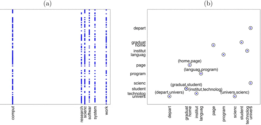
λ1= 0.45, λ2 = 0.25, andλ3 = 1.5.6 The estimated matrices are shown in Figure 8.

Figure 8(a) indicates that six hub nodes are detected: comput,research,scienc,software,

system, andwork. For instance, the fact that comput is a hub indicates that many terms’

occurrences are explained by the occurrence of the wordcomput. From Figure 8(b), we see that several pairs of terms take on non-zero values in the matrix (Z−diag(Z)). These include

(depart, univers);(home, page);(institut, technolog);(graduat, student);(univers, scienc),

and (languag,program). These results provide an intuitive explanation of the relationships

among the terms in the webpages.

(a) (b)

comput

research

scienc _softw

ar

system

w

or

k

depart

graduat home institut languag

page

program

scienc student technolog univers

depar

t

gr

aduat home _institut

languag

page

progr

am

scienc _student

technolog

univ

ers

●

(depart,univers)

●

(languag,program)

●

(home,page)

●

(graduat,student)

● ●

(institut,technolog)

●

(univers,scienc)

●

●

● ●

●

●

Figure 8: Results for HGL on the webpage data with tuning parameters selected using BIC:

λ1 = 0.45, λ2 = 0.25, λ3 = 1.5. Non-zero estimated values are shown, for (a):

(V−diag(V)), and (b): (Z−diag(Z)).

6.2 Application to Gene Expression Data

We applied HGL to a publicly available cancer gene expression data set (Verhaak et al., 2010). The data set consists of mRNA expression levels for 17,814 genes in 401 patients with glioblastoma multiforme (GBM), an extremely aggressive cancer with very poor patient prognosis. Among 7,462 genes known to be associated with cancer (Rappaport et al., 2013), we selected 500 genes with the highest variance.

We aim to reconstruct the gene regulatory network that represents the interactions among the genes, as well as to identify hub genes that tend to have many interactions with other genes. Such genes likely play an important role in regulating many other genes in the network. Identifying such regulatory genes will lead to a better understanding of brain cancer, and eventually may lead to new therapeutic targets. Since we are interested in identifying hub genes, and not as interested in identifying edges between non-hub nodes, we fix λ1 = 0.6 such that the matrix Z is sparse. We fix λ3 = 6.5 to obtain a few hub

nodes, and we select λ2 ranging from 0.1 to 0.7 using the BIC-type criterion presented in

We applied HGL with this set of tuning parameters to the empirical covariance matrix corresponding to the 401×500 data matrix, after standardizing each gene to have variance one. In Figure 9, we plotted the resulting network (for simplicity, only the 438 genes with at least two neighbors are displayed). We found that five genes are identified as hubs. These genes are TRIM48, TBC1D2B, PTPN2, ACRC, and ZNF763, in decreasing order of estimated edges.

Interestingly, some of these genes have known regulatory roles. PTPN2 is known to be a signaling molecule that regulates a variety of cellular processes including cell growth, differentiation, mitotic cycle, and oncogenic transformation (Maglott et al., 2004). ZNF763 is a DNA-binding protein that regulates the transcription of other genes (Maglott et al., 2004). These genes do not appear to be highly-connected to many other genes in the estimate that results from applying the graphical lasso (5) to this same data set (results not shown). These results indicate that HGL can be used to recover known regulators, as well as to suggest other potential regulators that may be targets for follow-up analysis.

1

3 5

4

2

2 4 6 8 10

2

4

6

8

10

1:10

1:10

1 - TRIM48 2 - TBC1D2B 3 - PTPN2 4 - ACRC 5 - ZNF763

Figure 9: Results for HGL on the GBM data with tuning parameters selected using BIC:

λ1 = 0.6,λ2 = 0.4,λ3= 6.5. Only nodes with at least two edges in the estimated

network are displayed. Nodes displayed in pink were found to be hubs by the HGL algorithm.

7. Discussion