Order-Independent Constraint-Based Causal Structure
Learning
Diego Colombo [email protected]
Marloes H. Maathuis [email protected]
Seminar for Statistics ETH Zurich
8092 Zurich, Switzerland
Editor:Peter Spirtes
Abstract
We consider constraint-based methods for causal structure learning, such as the PC-, FCI-, RFCI- and CCD- algorithms (Spirtes et al., 1993, 2000; Richardson, 1996; Colombo et al., 2012; Claassen et al., 2013). The first step of all these algorithms consists of the adja-cency search of the PC-algorithm. The PC-algorithm is known to be order-dependent, in the sense that the output can depend on the order in which the variables are given. This order-dependence is a minor issue in low-dimensional settings. We show, however, that it can be very pronounced in high-dimensional settings, where it can lead to highly variable results. We propose several modifications of the PC-algorithm (and hence also of the other algorithms) that remove part or all of this order-dependence. All proposed modifications are consistent in high-dimensional settings under the same conditions as their original counterparts. We compare the PC-, FCI-, and RFCI-algorithms and their mod-ifications in simulation studies and on a yeast gene expression data set. We show that our modifications yield similar performance in low-dimensional settings and improved
per-formance in high-dimensional settings. All software is implemented in the R-packagepcalg.
Keywords: directed acyclic graph, PC-algorithm, FCI-algorithm, CCD-algorithm, order-dependence, consistency, high-dimensional data
1. Introduction
Constraint-based methods for causal structure learning use conditional independence tests to obtain information about the underlying causal structure. We start by discussing several prominent examples of such algorithms, designed for different settings.
The PC-algorithm (Spirtes et al., 1993, 2000) was designed for learning directed acyclic
graphs (DAGs) under the assumption of causal sufficiency, i.e., no unmeasured common
causes and no selection variables. It learns a Markov equivalence class of DAGs that can be uniquely described by a so-called completed partially directed acyclic graph (CPDAG) (see Section 2 for a precise definition). The PC-algorithm is widely used in high-dimensional settings (Kalisch et al., 2010; Nagarajan et al., 2010; Stekhoven et al., 2012; Zhang et al., 2012), since it is computationally feasible for sparse graphs with up to thousands of variables, and open-source software is available, for example in TETRAD IV (Spirtes et al., 2000) and
to be consistent for high-dimensional sparse graphs (Kalisch and B¨uhlmann, 2007; Harris and Drton, 2013).
The FCI- and RFCI-algorithms and their modifications (Spirtes et al., 1993, 2000, 1999; Spirtes, 2001; Zhang, 2008; Colombo et al., 2012; Claassen et al., 2013) were designed for
learning directedacyclicgraphs whenallowing for latent and selection variables. Thus, these
algorithms learn a Markov equivalence class of DAGs with latent and selection variables, which can be uniquely represented by a partial ancestral graph (PAG). These algorithms first employ the adjacency search of the PC-algorithm, and then perform additional conditional independence tests because of the latent variables.
Finally, the CCD-algorithm (Richardson, 1996) was designed for learning Markov
equiv-alence classes of directed (not necessarily acyclic) graphs under the assumption of causal
sufficiency. Again, the first step of this algorithm consists of the adjacency search of the PC-algorithm.
Hence, all these algorithms share the adjacency search of the PC-algorithm as a common first step. We will therefore focus our analysis on this algorithm, since any improvements to the algorithm can be directly carried over to the other algorithms. When the PC-algorithm is applied to data, it is generally order-dependent, in the sense that its output depends on the order in which the variables are given. Dash and Druzdzel (1999) exploit the order-dependence to obtain candidate graphs for a score-based approach. Cano et al. (2008) resolve the order-dependence via a rather involved method based on measuring edge strengths. Spirtes et al. (2000) (Section 5.4.2.4) propose a method that removes the “weak-est” edges as early as possible. Overall, however, the order-dependence of the PC-algorithm has received relatively little attention in the literature, suggesting that it seems to be re-garded as a minor issue. We found, however, that the order-dependence can become very problematic for high-dimensional data, leading to highly variable results and conclusions for different variable orderings.
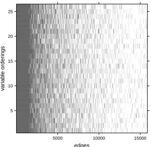
In particular, we analyzed the yeast gene expression data set of Hughes et al. (2000). We chose these data, despite the existence of larger and newer yeast gene expression data sets, since these data contain both observational and experimental data, obtained under similar conditions. The observational data consist of gene expression levels of 5361 genes for 63 wild-type yeast organisms, and the experimental data consist of gene expression levels of the same 5361 genes for 234 single-gene knockout strains. Hence, these data form a nice test bed for causal inference: algorithms can be applied to the observational data, and their output can be compared to the “gold standard” experimental data. (Please see Section 6 for more detailed information about the data.)
An important motivation for learning DAGs lies in their causal interpretation. We therefore also investigated the effect of different variable orderings on causal inference that is based on the PC-algorithm. In particular, we applied the IDA algorithm (Maathuis et al., 2010, 2009) to the observational yeast gene expression data, for 25 random variable orderings. The IDA algorithm conceptually consists of two-steps: one first estimates the Markov equivalence class of DAGs using the PC-algorithm, and one then applies Pearl’s do-calculus (Pearl, 2000) to each DAG in the Markov equivalence class. (The algorithm uses a fast local implementation that does not require listing all DAGs in the equivalence class.) One can then obtain estimated lower bounds on the sizes of the causal effects between all pairs of genes. For each of the 25 random variable orderings, we ranked the gene pairs according to these lower bounds, and compared these rankings to a gold standard set of large causal effects computed from the experimental single gene knock-out data, as in Maathuis et al. (2010). Figure 1(b) shows the large variability in the resulting receiver operating characteristic (ROC) curves. The ROC curve that was published in Maathuis et al. (2010)
was significantly better than random guessing with p < 0.001, and is somewhere in the
middle. Some of the other curves are much better, while there are also curves that are indistinguishable from random guessing.
The remainder of the paper is organized as follows. In Section 2 we discuss some back-ground and terminology. Section 3 explains the original PC-algorithm. Section 4 introduces modifications of the PC-algorithm (and hence also of the (R)FCI- and CCD-algorithms) that remove part or all of the order-dependence. These modifications are identical to their original counterparts when perfect conditional independence information is used. When applied to data, the modified algorithms are partly or fully order-independent. Moreover, they are consistent in high-dimensional settings under the same conditions as the original algorithms. Section 5 compares all algorithms in simulations, and Section 6 compares them on the yeast gene expression data discussed above. We close with a discussion in Section 7.
2. Preliminaries
In this section, we introduce some necessary terminology and background information.
2.1 Graph Terminology
A graph G = (V,E) consists of a vertex set V = {X1, . . . , Xp} and an edge set E. The
vertices represent random variables and the edges represent relationships between pairs of variables.
A graph containing only directed edges (→) is directed, one containing only undirected
edges (−) is undirected, and one containing directed and/or undirected edges is partially
directed. The skeleton of a partially directed graph is the undirected graph that results when all directed edges are replaced by undirected edges.
All graphs we consider aresimple, meaning that there is at most one edge between any
pair of vertices. If an edge is present, the vertices are said to be adjacent. If all pairs of
vertices in a graph are adjacent, the graph is calledcomplete. Theadjacency set of a vertex
Xi in a graph G = (V,E), denoted by adj(G, Xi), is the set of all vertices in V that are
adjacent to Xi in G. A vertex Xj in adj(G, Xi) is called a parent of Xi if Xj → Xi. The
edges
v
ar
iab
le order
ings
5 10 15 20 25
5000 10000 15000
(a) Edges occurring in the estimated skele-tons for 25 random variable orderings, as well as for the original ordering (shown as variable ordering 26). A black entry for an
edgeiand a variable orderingjmeans that
edgeioccurred in the estimated skeleton
for thejth variable ordering. The edges
along thex-axis are ordered according to
their frequency of occurrence in the esti-mated skeletons, from edges that occurred always to edges that occurred only once. Edges that did not occur for any of the variable orderings were omitted. For tech-nical reasons, only every 10th edge is ac-tually plotted.
False positives
0 1000 2000 3000 4000 0
200 400 600 800 1000 1200 1400 1600 1800 2000 2200 2400
T
rue positiv
es
(b) ROC curves corresponding to the 25 ran-dom orderings of the variables (solid black), where the curves are generated exactly as in Maathuis et al. (2010). The ROC curve for the original ordering of the variables (dashed blue) was published in Maathuis et al. (2010). The dashed-dotted red curve represents ran-dom guessing.
Figure 1: Analysis of the yeast gene expression data (Hughes et al., 2000) for 25 random
orderings of the variables, using tuning parameter α = 0.01. The estimated
graphs and resulting causal rankings are highly order-dependent.
Apathis a sequence of distinct adjacent vertices. Adirected pathis a path along directed
edges that follows the direction of the arrowheads. Adirected cycle is formed by a directed
path fromXi toXj together with the edgeXj →Xi. A (partially) directed graph is called
a (partially) directed acyclic graph if it does not contain directed cycles.
A triple (Xi, Xj, Xk) in a graphG is unshielded ifXi and Xj as well as Xj andXk are
adjacent, butXi andXkare not adjacent in G. Av-structure (Xi, Xj, Xk) is an unshielded
triple in a graph G where the edges are oriented as Xi →Xj ←Xk.
2.2 Probabilistic and Causal Interpretation of DAGs
We use the notation Xi ⊥⊥ Xj|S to indicate that Xi is independent of Xj given S, where
S is a set of variables not containing Xi and Xj (Dawid, 1980). If S is the empty set, we
separating setSfor (Xi, Xj) is calledminimal if there is no proper subsetS0 ofS such that
Xi⊥⊥Xj|S0.
A distributionQis said tofactorize according to a DAGG= (V,E) if the joint density
of V = (X1, . . . , Xp) can be written as the product of the conditional densities of each
variable given its parents in G: q(X1, . . . , Xp) =
Qp
i=1q(Xi|pa(G, Xi)).
A DAG entails conditional independence relationships via a graphical criterion called
d-separation (Pearl, 2000). If two vertices Xi and Xj are not adjacent in a DAG G, then
they are d-separated in G by a subset S of the remaining vertices. If Xi and Xj are
d-separated by S, then Xi ⊥⊥Xj|S in any distribution Q that factorizes according to G. A
distribution Qis said to be faithful to a DAG G if the reverse implication also holds, that
is, if the conditional independence relationships inQare exactly the same as those that can
be inferred from G using d-separation.
Several DAGs can describe exactly the same conditional independence information. Such DAGs are called Markov equivalent and form a Markov equivalence class. Markov equivalent DAGs have the same skeleton and the same v-structures, and a Markov equivalence class can be described uniquely by a completed partially directed acyclic graph (CPDAG) (Andersson et al., 1997; Chickering, 2002). A CPDAG is a partially directed acyclic graph with the following properties: every directed edge exists in every DAG in the Markov equivalence
class, and for every undirected edgeXi−Xj there exists a DAG withXi →Xj and a DAG
withXi←Xj in the Markov equivalence class. A CPDAGC is said to represent a DAGG
ifG belongs to the Markov equivalence class described by C.
A DAG can be interpreted causally in the following way (Pearl, 2000, 2009; Spirtes et al.,
2000): X1 is a direct cause of X2 only if X1 → X2, and X1 is a possibly indirect cause of
X2 only if there is a directed path from X1 toX2.
3. The PC-Algorithm
We now describe the PC-algorithm in detail. In Section 3.1, we discuss the algorithm under the assumption that we have perfect conditional independence information between
all variables inV. We refer to this as theoracle version. In Section 3.2 we discuss the more
realistic situation where conditional independence relationships have to be estimated from
data. We refer to this as the sample version.
3.1 Oracle Version
A sketch of the PC-algorithm is given in Algorithm 3.1. We see that the algorithm consists
of three steps. Step 1 (also calledadjacency search) finds the skeleton and separation sets,
while Steps 2 and 3 determine the orientations of the edges.
Step 1 is given in pseudo-code in Algorithm 3.2. We start with a complete undirected
graph C. This graph is subsequently thinned out in the loop on lines 3-15 in Algorithm
3.2, where an edge Xi−Xj is deleted if Xi ⊥⊥ Xj|S for some subset S of the remaining
variables. These conditional independence queries are organized in a way that makes the algorithm computationally efficient for high-dimensional sparse graphs, since we only need
to query conditional independencies up to order q−1, where q is the maximum size of the
Algorithm 3.1The PC-algorithm (oracle version)
Require: Conditional independence information among all variables inV, and an ordering
order(V) on the variables
1: Adjacency search: Find the skeletonC and separation sets using Algorithm 3.2;
2: Orient unshielded triples in the skeletonC based on the separation sets;
3: InCorient as many of the remaining undirected edges as possible by repeated application
of rules R1-R3 (see text);
4: return Output graph (C) and separation sets (sepset).
Algorithm 3.2Adjacency search / Step 1 of the PC-algorithm (oracle version)
Require: Conditional independence information among all variables inV, and an ordering
order(V) on the variables
1: Form the complete undirected graphC on the vertex set V
2: Let`=−1;
3: repeat
4: Let `=`+ 1;
5: repeat
6: Select a (new) ordered pair of vertices (Xi, Xj) that are adjacent in C and satisfy
|adj(C, Xi)\ {Xj}| ≥`, using order(V);
7: repeat
8: Choose a (new) setS⊆adj(C, Xi)\ {Xj} with|S|=`, using order(V);
9: if Xi and Xj are conditionally independent givenS then
10: Delete edge Xi−Xj from C;
11: Let sepset(Xi, Xj) = sepset(Xj, Xi) =S;
12: end if
13: until Xi and Xj are no longer adjacent in C or all S ⊆ adj(C, Xi)\ {Xj} with
|S|=`have been considered
14: until all ordered pairs of adjacent vertices (Xi, Xj) in C with|adj(C, Xi)\ {Xj}| ≥`
have been considered
15: untilall pairs of adjacent vertices (Xi, Xj) in C satisfy|adj(C, Xi)\ {Xj}| ≤`
First, when`= 0, all pairs of vertices are tested for marginal independence. IfXi⊥⊥Xj,
then the edgeXi−Xj is deleted and the empty set is saved as separation set in sepset(Xi, Xj)
and sepset(Xj, Xi). After all pairs of vertices have been considered (and many edges might
have been deleted), the algorithm proceeds to the next step with`= 1.
When ` = 1, the algorithm chooses an ordered pair of vertices (Xi, Xj) still adjacent
in C, and checks Xi ⊥⊥ Xj|S for subsets S of size ` = 1 of adj(C, Xi)\ {Xj}. If such a
conditional independence is found, the edge Xi −Xj is removed, and the corresponding
conditioning set S is saved in sepset(Xi, Xj) and sepset(Xj, Xi). If all ordered pairs of
adjacent vertices have been considered for conditional independence given all subsets of size
` of their adjacency sets, the algorithm again increases ` by one. This process continues
until all adjacency sets in the current graph are smaller than `. At this point the skeleton
and the separation sets have been determined.
We see that this procedure indeed ensures that we only query conditional independencies
up to order q−1, where q is the maximum size of the adjacency sets of the nodes in the
underlying DAG. This makes the algorithm particularly efficient for large sparse graphs. Step 2 determines the v-structures. In particular, it considers all unshielded triples
in C, and orients an unshielded triple (Xi, Xj, Xk) as a v-structure if and only if Xj ∈/
sepset(Xi, Xk).
Finally, Step 3 orients as many of the remaining undirected edges as possible by repeated application of the following three rules:
R1: orient Xj−Xk intoXj →Xk whenever there is a directed edge Xi → Xj such that
Xi and Xk are not adjacent (otherwise a new v-structure is created);
R2: orient Xi−Xj into Xi →Xj whenever there is a chainXi →Xk →Xj (otherwise a
directed cycle is created);
R3: orient Xi −Xj into Xi → Xj whenever there are two chains Xi −Xk → Xj and
Xi−Xl →Xj such thatXk andXl are not adjacent (otherwise a new v-structure or
a directed cycle is created).
The PC-algorithm was shown to be sound and complete.
Theorem 1 (Theorem 5.1 on p.410 of Spirtes et al., 2000) Let the distribution of V be faithful to a DAG G = (V,E), and assume that we are given perfect conditional indepen-dence information about all pairs of variables(Xi, Xj)in Vgiven subsetsS⊆V\ {Xi, Xj}.
Then the output of the PC-algorithm is the CPDAG that representsG.
We briefly discuss the main ingredients of the proof, as these will be useful for un-derstanding our modifications in Section 4. The faithfulness assumption implies that
con-ditional independence in the distribution of V is equivalent to d-separation in the graph
G. The skeleton of G can then be determined as follows: Xi and Xj are adjacent in G if
and only if they are conditionally dependent given any subset S of the remaining nodes.
Naively, one could therefore check all these conditional dependencies, which is known as the SGS-algorithm (Spirtes et al., 2000). The PC-algorithm obtains the same result with fewer
tests, by using the following fact about DAGs: two variables Xi and Xj in a DAG G are
by pa(G, Xi) or pa(G, Xj). The PC-algorithm is guaranteed to check these conditional
inde-pendencies: at all stages of the algorithm, the graphCis a supergraph of the true CPDAG,
and the algorithm checks conditional dependencies given all subsets of the adjacency sets, which obviously include the parent sets.
The v-structures are determined based on Lemmas 5.1.2 and 5.1.3 of Spirtes et al. (2000). The soundness and completeness of the orientation rules in Step 3 was shown in Meek (1995) and Andersson et al. (1997).
3.2 Sample Version
In applications, we of course do not have perfect conditional independence information.
Instead, we assume that we have an i.i.d. sample of size nof V= (X1, . . . , Xp). A sample
version of the PC-algorithm can then be obtained by replacing all conditional independence queries by statistical conditional independence tests at some pre-specified significance level
α. For example, if the distribution ofVis multivariate Gaussian, one can test for zero partial
correlation, see, e.g., Kalisch and B¨uhlmann (2007). This is the test we used throughout
this paper.
We note that the PC-algorithm performs many tests. Hence,αshould not be interpreted
as an overall significance level. Rather, it plays the role of a tuning parameter, where smaller
values ofα tend to lead to sparser graphs.
3.3 Order-Dependence in the Sample Version
Let order(V) denote an ordering on the variables in V. We now consider the role of
order(V) in every step of the algorithm. Throughout, we assume that all tasks are performed
according to the lexicographical ordering of order(V), which is the standard implementation
inpcalg(Kalisch et al., 2012) and TETRAD IV (Spirtes et al., 2000), and is called “PC-1” in Spirtes et al. (2000) (Section 5.4.2.4).
In Step 1, order(V) affects the estimation of the skeleton and the separating sets. In
particular, at each level of `, order(V) determines the order in which pairs of adjacent
vertices and subsetsSof their adjacency sets are considered (see lines 6 and 8 in Algorithm
3.2). The skeletonCis updated after each edge removal. Hence, the adjacency sets typically
change within one level of `, and this affects which other conditional independencies are
checked, since the algorithm only conditions on subsets of the adjacency sets. In the oracle version, we have perfect conditional independence information, and all orderings on the variables lead to the same output. In the sample version, however, we typically make mistakes in keeping or removing edges. In such cases, the resulting changes in the adjacency sets can lead to different skeletons, as illustrated in Example 1.
Moreover, different variable orderings can lead to different separating sets in Step 1. In the oracle version, this is not important, because any valid separating set leads to the correct v-structure decision in Step 2. In the sample version, however, different separating sets in Step 1 of the algorithm may yield different decisions about v-structures in Step 2. This is illustrated in Example 2.
Finally, we consider the role of order(V) on the orientation rules in Steps 2 and 3
orderings can lead to different orientations, even if the skeleton and separating sets are order-independent.
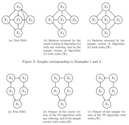
Example 1 (Order-dependent skeleton in the sample version of the PC-algorithm.) Sup-pose that the distribution of V = {X1, X2, X3, X4, X5} is faithful to the DAG in Figure
2(a). This DAG encodes the following conditional independencies with minimal separating sets: X1 ⊥⊥X2 andX2 ⊥⊥X4|{X1, X3} .
Suppose that we have an i.i.d. sample of (X1, X2, X3, X4, X5), and that the following
conditional independencies with minimal separating sets are judged to hold at some signifi-cance level α: X1 ⊥⊥X2, X2 ⊥⊥X4|{X1, X3}, and X3 ⊥⊥X4|{X1, X5}. Thus, the first two
are correct, while the third is false.
We now apply the PC-algorithm with two different orderings: order1(V) = (X1, X4, X2,
X3, X5) and order2(V) = (X1, X3, X4, X2, X5). The resulting skeletons are shown in
Fig-ures 2(b) and 2(c), respectively. We see that the skeletons are different, and that both are incorrect as the edgeX3−X4 is missing. The skeleton for order2(V) contains an additional
error, as there is an additional edge X2−X4.
We now go through Algorithm 3.2 to see what happened. We start with a complete undi-rected graph on V. When ` = 0, variables are tested for marginal independence, and the algorithm correctly removes the edge betweenX1 and X2. No other conditional
independen-cies are found when ` = 0 or `= 1. When ` = 2, there are two pairs of vertices that are thought to be conditionally independent given a subset of size 2, namely the pairs (X2, X4)
and (X3, X4).
In order1(V), the pair (X4, X2) is considered first. The corresponding edge is removed,
as X4 ⊥⊥ X2|{X1, X3} and {X1, X3} is a subset of adj(C, X4) = {X1, X2, X3, X5}. Next,
the pair(X4, X3) is considered and the corresponding edges is erroneously removed, because
of the wrong decision that X4 ⊥⊥ X3|{X1, X5} and the fact that {X1, X5} is a subset of
adj(C, X4) ={X1, X3, X5}.
In order2(V), the pair (X3, X4) is considered first, and the corresponding edge is
er-roneously removed. Next, the algorithm considers the pair (X4, X2). The corresponding
separating set {X1, X3} is not a subset of adj(C, X4) = {X1, X2, X5}, so that the edge
X2−X4 remains. Next, the algorithm considers the pair (X2, X4). Again, the separating
set {X1, X3} is not a subset of adj(C, X2) ={X3, X4, X5}, so that the edge X2−X4 again
remains. In other words, since (X3, X4) was considered first in order2(V), the adjacency
set of X4 was affected and no longer contained X3, so that the algorithm “forgot” to check
the conditional independence X2 ⊥⊥X4|{X1, X3}.
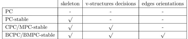
Example 2 (Order-dependent separating sets and v-structures in the sample version of the PC-algorithm.) Suppose that the distribution of V = {X1, X2, X3, X4, X5} is faithful to
the DAG in Figure 3(a). This DAG encodes the following conditional independencies with minimal separating sets: X1 ⊥⊥X3|{X2},X1⊥⊥X4|{X2},X1 ⊥⊥X4|{X3}, X2 ⊥⊥X4|{X3},
X2⊥⊥X5|{X1, X3}, X2⊥⊥X5|{X1, X4}, X3 ⊥⊥X5|{X1, X4} and X3 ⊥⊥X5|{X2, X4}.
We consider the oracle version of the PC-algorithm with two different orderings on the variables: order3(V) = (X1, X4, X2, X3, X5) and order4(V) = (X1, X4, X3, X2, X5). For
{X3}. Thus, the separating sets are order-dependent. However, we obtain the same
v-structure X1 → X5 ← X4 for both orderings, since X5 is not in the sepset(X1, X4),
re-gardless of the ordering. In fact, this holds in general, since in the oracle version of the PC-algorithm, a vertex is either in all possible separating sets or in none of them (Spirtes et al., 2000, Lemma 5.1.3).
Now suppose that we have an i.i.d. sample of (X1, X2, X3, X4, X5). Suppose that at
some significance levelα, all true conditional independencies are judged to hold, and X1⊥
⊥ X3|{X4} is thought to hold by mistake. We again consider two different orderings:
order5(V) = (X1, X3, X4, X2, X5) and order6(V) = (X3, X1, X2, X4, X5). With order5(V)
we obtain the incorrect sepset(X1, X3) = {X4}. This also leads to an incorrect v-structure
X1 → X2 ← X3 in Step 2 of the algorithm. With order6(V), we obtain the correct
sepset(X1, X3) ={X2}, and hence correctly find thatX1−X2−X3 is not a v-structure in
Step 2. This illustrates that order-dependent separating sets in Step 1 of the sample version of the PC-algorithm can lead to order-dependent v-structures in Step 2 of the algorithm.
Example 3 (Order-dependent orientation rules in Steps 2 and 3 of the sample version of the PC-algorithm.) Consider the graph in Figure 4(a) with unshielded triples (X1, X2, X3)
and (X2, X3, X4), and assume this is the skeleton after Step 1 of the sample version of
the PC-algorithm. Moreover, assume that we found sepset(X1, X3) = sepset(X2, X4) =
sepset(X1, X4) = ∅. Then in Step 2 of the algorithm, we obtain two v-structures X1 →
X2←X3 andX2 →X3←X4. Of course this means that at least one of the statistical tests
is wrong, but this can happen in the sample version. We now have conflicting information about the orientation of the edge X2−X3. In the current implementation of pcalg, where
conflicting edges are simply overwritten, this means that the orientation of X2 −X3 is
determined by the v-structure that is last considered. Thus, we obtainX1→X2→X3←X4
if (X2, X3, X4) is considered last, while we get X1 → X2 ← X3 ← X4 if (X1, X2, X3) is
considered last.
Next, consider the graph in Figure 4(b), and assume that this is the output of the sam-ple version of the PC-algorithm after Step 2. Thus, we have two v-structures, namely
X1 → X2 ← X3 and X4 → X5 ← X6, and four unshielded triples, namely (X1, X2, X5),
(X3, X2, X5), (X4, X5, X2), and (X6, X5, X2). Thus, we then apply the orientation rules
in Step 3 of the algorithm, starting with rule R1. If one of the two unshielded triples
(X1, X2, X5) or(X3, X2, X5) is considered first, we obtain X2 →X5. On the other hand, if
one of the unshielded triples (X4, X5, X2) or(X6, X5, X2) is considered first, then we obtain
X2←X5. Note that we have no issues with overwriting of edges here, since as soon as the
edgeX2−X5 is oriented, all edges are oriented and no further orientation rules are applied.
These examples illustrate that Steps 2 and 3 of the PC-algorithm can be order-dependent regardless of the output of the previous steps.
4. Modified Algorithms
X1 X2
X3
X4
X5
(a) True DAG.
X1 X2
X3
X4
X5
(b) Skeleton returned by the oracle version of Algorithm 3.2 with any ordering, and by the sample version of Algorithm
3.2 with order1(V).
X1 X2
X3
X4
X5
(c) Skeleton returned by the sample version of Algorithm
3.2 with order2(V).
Figure 2: Graphs corresponding to Examples 1 and 4.
X1
X2 X3
X4
X5
(a) True DAG.
X1
X2 X3
X4
X5
(b) Output of the oracle ver-sion of the PC-algorithm with any ordering, and of the sample
version with order6(V).
X1
X2 X3
X4
X5
(c) Output of the sample ver-sion of the PC-algorithm with
order5(V).
Figure 3: Graphs corresponding to Examples 2 and 5.
X1
X2 X3
X4
(a) Possible skeleton after Step 1 of the sample version of the PC-algorithm.
X2
X3 X4
X5
X1 X6
(b) Possible partially directed graph af-ter Step 2 of the sample version of the PC-algorithm.
results and examples about order-dependence in the corresponding sample version (obtained by replacing conditional independence queries by conditional independence tests, as in Sec-tion 3.3). Finally, SecSec-tion 4.4 discusses order-independent versions of related algorithms like RFCI and FCI, and Section 4.5 presents high-dimensional consistency results for the sample versions of all modifications.
4.1 The Skeleton
We first consider estimation of the skeleton in the adjacency search (Step 1) of the PC-algorithm. The pseudocode for our modification is given in Algorithm 4.1. The resulting PC-algorithm, where Step 1 in Algorithm 3.1 is replaced by Algorithm 4.1, is called “PC-stable”.
The main difference between Algorithms 3.2 and 4.1 is given by the for-loop on lines
6-8 in the latter one, which computes and stores the adjacency sets a(Xi) of all variables
after each new size ` of the conditioning sets. These stored adjacency setsa(Xi) are used
whenever we search for conditioning sets of this given size`. Consequently, an edge deletion
on line 13 no longer affects which conditional independencies are checked for other pairs of
variables at this level of `.
In other words, at each level of`, Algorithm 4.1 records which edges should be removed,
but for the purpose of the adjacency sets it removes these edges only when it goes to the
next value of `. Besides resolving the order-dependence in the estimation of the skeleton,
our algorithm has the advantage that it is easily parallelizable at each level of `.
The PC-stable algorithm is sound and complete in the oracle version (Theorem 2), and yields order-independent skeletons in the sample version (Theorem 3). We illustrate the algorithm in Example 4.
Theorem 2 Let the distribution ofV be faithful to a DAGG= (V,E), and assume that we are given perfect conditional independence information about all pairs of variables(Xi, Xj)
in V given subsets S ⊆ V\ {Xi, Xj}. Then the output of the PC-stable algorithm is the
CPDAG that representsG.
Proof The proof of Theorem 2 is completely analogous to the proof of Theorem 1 for the original PC-algorithm, as discussed in Section 3.1.
Theorem 3 The skeleton resulting from the sample version of the PC-stable algorithm is order-independent.
Proof We consider the removal or retention of an arbitrary edgeXi−Xj at some level`.
The ordering of the variables determines the order in which the edges (line 9 of Algorithm
4.1) and the subsets S of a(Xi) and a(Xj) (line 11 of Algorithm 4.1) are considered. By
construction, however, the order in which edges are considered does not affect the setsa(Xi)
and a(Xj).
If there is at least one subset S of a(Xi) or a(Xj) such that Xi ⊥⊥ Xj|S, then any
ordering of the variables will find a separating set for Xi and Xj (but different orderings
Algorithm 4.1Step 1 of the PC-stable algorithm (oracle version)
Require: Conditional independence information among all variables inV, and an ordering
order(V) on the variables
1: Form the complete undirected graphC on the vertex set V
2: Let`=−1;
3: repeat
4: Let `=`+ 1;
5: for allvertices Xi inC do
6: Leta(Xi) = adj(C, Xi)
7: end for
8: repeat
9: Select a (new) ordered pair of vertices (Xi, Xj) that are adjacent in C and satisfy
|a(Xi)\ {Xj}| ≥`, using order(V);
10: repeat
11: Choose a (new) setS⊆a(Xi)\ {Xj} with|S|=`, using order(V);
12: if Xi and Xj are conditionally independent givenS then
13: Delete edge Xi−Xj from C;
14: Let sepset(Xi, Xj) = sepset(Xj, Xi) =S;
15: end if
16: untilXi and Xj are no longer adjacent in C or allS ⊆a(Xi)\ {Xj}with |S|=`
have been considered
17: untilall ordered pairs of adjacent vertices (Xi, Xj) inCwith|a(Xi)\ {Xj}| ≥`have
been considered
18: untilall pairs of adjacent vertices (Xi, Xj) in C satisfy|a(Xi)\ {Xj}| ≤`
19: return C, sepset.
subsetS0 of a(Xi) or a(Xj) such that Xi ⊥⊥Xj|S0, then no ordering will find a separating
set.
Hence, any ordering of the variables leads to the same edge deletions, and therefore to the same skeleton.
Example 4 (Order-independent skeletons) We go back to Example 1, and consider the sample version of Algorithm 4.1. The algorithm now outputs the skeleton shown in Figure 2(b) for both orderings order1(V) and order2(V).
We again go through the algorithm step by step. We start with a complete undirected graph on V. The only conditional independence found when ` = 0 or `= 1 is X1 ⊥⊥X2,
and the corresponding edge is removed. When `= 2, the algorithm first computes the new adjacency sets: a(X1) = a(X2) = {X3, X4, X5} and a(Xi) = V \ {Xi} for i = 3,4,5.
There are two pairs of variables that are thought to be conditionally independent given a subset of size 2, namely (X2, X4) and (X3, X4). Since the sets a(Xi) are not updated after
edge removals, it does not matter in which order we consider the ordered pairs (X2, X4),
separating set {X1, X3} for(X4, X2)is contained in a(X4), and the separating set{X1, X5}
for (X3, X4) is contained in a(X3) (and in a(X4)).
4.2 Determination of the V-structures
We propose two methods to resolve the order-dependence in the determination of the v-structures, using the conservative PC-algorithm (CPC) of Ramsey et al. (2006) and a vari-ation thereof.
The CPC-algorithm works as follows. LetCbe the graph resulting from Step 1 of the
PC-algorithm (Algorithm 3.1). For all unshielded triples (Xi, Xj, Xk) inC, determine all subsets
Yof adj(C, Xi) and of adj(C, Xk) that makeXi andXkconditionally independent, i.e., that
satisfy Xi ⊥⊥ Xk|Y. We refer to such sets as separating sets. The triple (Xi, Xj, Xk) is
labelled as unambiguous if at least one such separating set is found and eitherXj is in all
separating sets or in none of them; otherwise it is labelled as ambiguous. If the triple is
unambiguous, it is oriented as v-structure if and only if Xj is in none of the separating
sets. Moreover, in Step 3 of the PC-algorithm (Algorithm 3.1), the orientation rules are adapted so that only unambiguous triples are oriented. The output of the CPC-algorithm is a partially directed graph in which ambiguous triples are marked.
We found that the CPC-algorithm can be very conservative, in the sense that very few unshielded triples are unambiguous in the sample version. We therefore propose a minor modification of this approach, called majority rule PC-algorithm (MPC). As in CPC, we
first determine all subsets Y of adj(C, Xi) and of adj(C, Xk) satisfying Xi ⊥⊥ Xk|Y. We
then label the triple (Xi, Xj, Xk) asunambiguous if at least one such separating set is found
and Xj is not in exactly 50% of the separating sets. Otherwise it is labelled as ambiguous.
(Of course, one can also use different cut-offs to declare ambiguous and non-ambiguous
triples.) If a triple is unambiguous, it is oriented as v-structure if and only if Xj is in less
than half of the separating sets. As in CPC, the orientation rules in Step 3 are adapted so that only unambiguous triples are oriented, and the output is a partially directed graph in which ambiguous triples are marked.
We refer to the combination of PC-stable and CPC/MPC as the CPC/MPC-stable algorithms. Theorem 4 states that the oracle versions of the CPC- and MPC-stable algo-rithms are sound and complete. When looking at the sample versions of the algoalgo-rithms, we note that any unshielded triple that is judged to be unambiguous in CPC-stable is also unambiguous in MPC-stable, and any unambiguous v-structure in CPC-stable is an unam-biguous v-structure in MPC-stable. In this sense, CPC-stable is more conservative than MPC-stable, although the difference appears to be small in simulations and for the yeast data (see Sections 5 and 6). Both CPC-stable and MPC-stable share the property that the determination of v-structures no longer depends on the (order-dependent) separating sets that were found in Step 1 of the algorithm. Therefore, both CPC-stable and MPC-stable yield order-independent decisions about v-structures in the sample version, as stated in Theorem 5. Example 5 illustrates both algorithms.
We note that the CPC/MPC-stable algorithms may yield a lot fewer directed edges than PC-stable. On the other hand, we can put more trust in those edges that were oriented.
inVgiven subsetsS⊆V\ {Xi, Xj}. Then the output of the CPC/MPC(-stable) algorithms
is the CPDAG that represents G.
Proof The skeleton of the CPDAG is correct by Theorems 1 and 2. The unshielded triples are all unambiguous (in the conservative and the majority rule versions), since for any
un-shielded triple (Xi, Xj, Xk) in a DAG,Xj is either in all sets that d-separate Xi and Xkor
in none of them (Spirtes et al., 2000, Lemma 5.1.3). In particular, this also means that all v-structures are determined correctly. Finally, since all unshielded triples are unambiguous, the orientation rules are as in the original oracle PC-algorithm, and soundness and com-pleteness of these rules follows from Meek (1995) and Andersson et al. (1997).
Theorem 5 The decisions about v-structures in the sample versions of the CPC/MPC-stable algorithms are order-independent.
Proof The CPC/MPC-stable algorithms have order-independent skeletons in Step 1, by
Theorem 3. In particular, this means that their unshielded triples and adjacency sets
are order-independent. The decision about whether an unshielded triple is unambiguous and/or a v-structure is based on the adjacency sets of nodes in the triple, which are order-independent.
Example 5 (Order-independent decisions about v-structures) We consider the sample ver-sions of the CPC/MPC-stable algorithms, using the same input as in Example 2. In par-ticular, we assume that all conditional independencies induced by the DAG in Figure 3(a) are judged to hold, plus the additional (erroneous) conditional independencyX1 ⊥⊥X3|X4.
Denote the skeleton after Step 1 by C. We consider the unshielded triple (X1, X2, X3).
First, we compute adj(C, X1) ={X2, X5} and adj(C, X3) ={X2, X4}. We now consider all
subsetsY of these adjacency sets, and check whetherX1 ⊥⊥X3|Y. The following separating
sets are found: {X2}, {X4}, and {X2, X4}.
SinceX2 is in some but not all of these separating sets, CPC-stable determines that the
triple is ambiguous, and no orientations are performed. SinceX2 is in more than half of the
separating sets, MPC-stable determines that the triple is unambiguous and not a v-structure. The output of both algorithms is given in Figure 3(b).
4.3 Orientation Rules
Even when the skeleton and the determination of the v-structures are order-independent, Example 3 showed that there might be some order-dependence left in the sample-version.
This can be resolved by allowing bi-directed edges (↔) and working with lists containing
the candidate edges for the v-structures in Step 2 and the orientation rules R1-R3 in Step 3.
these edges, again creating bi-directed edges if there are conflicts. We do the same for rules R2 and R3, and iterate this procedure until no more edges can be oriented.
When using this procedure, we add the letter L (standing for lists), e.g., LCPC-stable and LMPC-stable. The LCPC-stable and LMPC-stable algorithms are correct in the oracle version (Theorem 6) and fully order-independent in the sample versions (Theorem 7). The procedure is illustrated in Example 6.
We note that the bi-directed edges cannot be interpreted causally. They simply indicate that there was some conflicting information in the algorithm.
Theorem 6 Let the distribution ofV be faithful to a DAGG= (V,E), and assume that we are given perfect conditional independence information about all pairs of variables(Xi, Xj)
in V given subsets S ⊆ V\ {Xi, Xj}. Then the (L)CPC(-stable) and (L)MPC(-stable)
algorithms output the CPDAG that represents G.
Proof By Theorem 4, we know that the CPC(-stable) and MPC(-stable) algorithms are correct. With perfect conditional independence information, there are no conflicts between v-structures in Step 2 of the algorithms, nor between orientation rules in Step 3 of the algorithms. Therefore, the (L)CPC(-stable) and (L)MPC(-stable) algorithms are identical to the CPC(-stable) and MPC(-stable) algorithms.
Theorem 7 The sample versions of LCPC-stable and LMPC-stable are fully order-indepen-dent.
Proof This follows straightforwardly from Theorems 3 and 5 and the procedure with lists and bi-directed edges discussed above.
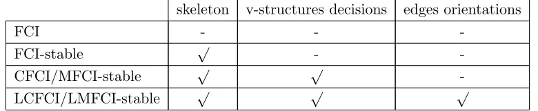
Table 1 summarizes the three order-dependence issues explained above and the cor-responding modifications of the PC-algorithm that removes the given order-dependence problem.
skeleton v-structures decisions edges orientations
PC - -
-PC-stable √ -
-CPC/MPC-stable √ √
-BCPC/BMPC-stable √ √ √
Example 6 First, we consider the two unshielded triples (X1, X2, X3)and(X2, X3, X4) as
shown in Figure 4(a). The version of the algorithm that uses lists for the orientation rules, orients these edges as X1→X2↔X3←X4, regardless of the ordering of the variables.
Next, we consider the structure shown in Figure 4(b). As a first step, we construct a list containing all candidate structures eligible for orientation rule R1 in Step 3. The list contains the unshielded triples (X1, X2, X5),(X3, X2, X5), (X4, X5, X2), and (X6, X5, X2).
Now, we go through each element in the list and we orient the edges accordingly, allowing bi-directed edges. This yields the edge orientation X2 ↔ X5, regardless of the ordering of
the variables.
4.4 Related Algorithms
If there are unmeasured common causes or unmeasured selection variables, which is often the case in practice, then causal inference based on the PC-algorithm may be incorrect. In such cases, one needs a generalization of a DAG, called a maximal ancestral graph (MAG) (Richardson and Spirtes, 2002). A MAG describes causal information in its edge
marks, and entails conditional independence relationships via m-separation (Richardson
and Spirtes, 2002), a generalization of d-separation. Several MAGs can describe exactly the same conditional independence information. Such MAGs are called Markov equivalent and form a Markov equivalence class, which can be represented by a partial ancestral graph (PAG) (Richardson and Spirtes, 2002; Ali et al., 2009). PAGs describe causal features common to every MAG in the Markov equivalence class, and hence to every DAG (possibly with latent and selection variables) compatible with the observable independence structure under the assumption of faithfulness. More information on the interpretation of MAGs and PAGs can be found in, e.g., Colombo et al. (2012) (Sections 1.2 and 2.2).
PAGs can be learned by the FCI-algorithm (Spirtes et al., 2000, 1999). As a first step, this algorithm runs Steps 1 and 2 of the PC-algorithm (Algorithm 3.1). Based on the resulting graph, it then computes certain sets, called “Possible-D-SEP” sets, and conducts more conditional independence tests given subsets of the Possible-D-SEP sets. This can lead to additional edge removals and corresponding separating sets. After this, the v-structures are newly determined. Finally, there are ten orientation rules as defined by Zhang (2008). The output of the FCI-algorithm is an (estimated) PAG (Colombo et al., 2012, Definition 3.1).
From our results, it immediately follows that FCI with any of our modifications of the PC-algorithm is sound and complete in the oracle version. Moreover, we can easily
construct partially or fully order-independent sample versions as follows. To solve the
CFCI-stable and MFCI-stable, respectively. Regarding the orientation rules, we note that the FCI-algorithm does not suffer from conflicting v-structures (as shown in Figure 4(a)
for the PC-algorithm), because it orients edge marks and because bi-directed edges are
allowed. However, the ten orientation rules still suffer from order-dependence issues as in the PC-algorithm (see Example 3 and Figure 4(b)). To solve this problem, we can again use lists of candidate edges for each orientation rule as explained in the previous section about the PC-algorithm. We refer to these modifications as LCFCI-stable and LMFCI-stable, and they are fully order-independent in the sample version. However, since these ten orientation rules are more involved than the three for PC, using lists can be very slow for some rules, for example the one for discriminating paths.
Table 2 summarizes the three order-dependence issues for FCI and the corresponding modifications that remove them.
skeleton v-structures decisions edges orientations
FCI - -
-FCI-stable √ -
-CFCI/MFCI-stable √ √
-LCFCI/LMFCI-stable √ √ √
Table 2: Order-dependence issues and corresponding modifications of the FCI-algorithm that remove the problem. A tick mark indicates that the corresponding aspect of the graph is estimated order-independently in the sample version. For exam-ple, with FCI-stable the skeleton is estimated order-independently but not the v-structures and the edge orientations.
In the presences of latent and selection variables, one can also use the RFCI-algorithm (Colombo et al., 2012). This algorithm can be viewed as a compromise between PC and FCI, in the sense that its computational complexity is of the same order as PC, but its output can be interpreted causally without assuming causal sufficiency (but is slightly less informative than the output from FCI).
RFCI works as follows. It starts with the first step of PC. It then has a more involved Step 2 to determine the v-structures (Colombo et al., 2012, Lemma 3.1). In particular, for
any unshielded triple (Xi, Xj, Xk), it conducts additional tests to check if bothXi and Xj
andXj andXk are conditionally dependent given sepset(Xi, Xj)\ {Xj}found in Step 1. If
a conditional independence relationship is detected, the corresponding edge is removed and a minimal separating set is stored. The removal of an edge can create new unshielded triples or destroy some of them. Therefore, the algorithm works with lists to make sure that these actions are order-independent. On the other hand, if both conditional dependencies hold and
Xj is not in the separating set for (Xi, Xk), the triple is oriented as a v-structure. Finally,
From our results, it immediately follows that RFCI with any of our modifications of the PC-algorithm is correct in the oracle version, in the sense it outputs the true RFCI-PAG. Because of its more involved rules for v-structures and discriminating paths, one needs to make several adaptations to create a fully order-independent algorithm. For example, the additional conditional independence tests conducted for the v-structures are based on the separating sets found in Step 1. As already mentioned before (see Example 2) these separating sets are order-dependent, and therefore also the possible edge deletions based on them are dependent, leading to an dependent skeleton. To produce an order-independent skeleton one should use a similar approach to the conservative one for the v-structures to make the additional edge removals order-independent. Nevertheless, we can remove a large amount of the order-dependence in the skeleton by using the stable version for the skeleton as a first step. We refer to this modification as RFCI-stable. Note that this procedure does not produce a fully order-independent skeleton, but as shown in Section 5.2, it reduces the order-dependence considerably. Moreover, we can combine this modification with CPC or MPC on the final skeleton to reduce the order-dependence of the v-structures. We refer to these modifications as CRFCI-stable and MRFCI-stable. Finally, we can again use lists for the orientation rules as in the FCI-algorithm to reduce the order-dependence caused by the orientation rules.
Finally, in the presence of directed cycles, one can use the CCD-algorithm (Richardson, 1996). This algorithm can also be made order-independent using a similar approach.
4.5 High-Dimensional Consistency
The original PC-algorithm has been shown to be consistent for certain sparse
high-dimensio-nal graphs. In particular, Kalisch and B¨uhlmann (2007) proved consistency for multivariate
Gaussian distributions. More recently, Harris and Drton (2013) showed consistency for the broader class of Gaussian copulas when using rank correlations, under slightly different conditions.
These high-dimensional consistency results allow the DAGGand the number of observed
variables p in V to grow as a function of the sample size, so that p = pn, V = Vn =
(Xn,1, . . . , Xn,pn) and G =Gn. The corresponding CPDAGs that representGn are denoted
byCn, and the estimated CPDAGs using tuning parameterαnare denoted by ˆCn(αn). Then
the consistency results say that, under some conditions, there exists a sequenceαnsuch that
P( ˆCn(αn) =Cn)→1 asn→ ∞.
These consistency results rely on the fact that the PC-algorithm only performs
condi-tional independence tests between pairs of variables given subsetsSof size less than or equal
to the degree of the graph (when no errors are made). We made sure that our modifications
still obey this property, and therefore the consistency results of Kalisch and B¨uhlmann
(2007) and Harris and Drton (2013) remain valid for the (L)CPC(-stable) and (L)MPC(-stable) algorithms, under exactly the same conditions as for the original PC-algorithm.
5. Simulations
We compared all algorithms on simulated data from low-dimensional and high-dimensional systems with and without latent variables. In the low-dimensional setting, we compared the modifications of PC, FCI and RFCI. All algorithms performed similarly in this setting, and the results are presented in Appendix A.1. The remainder of this section therefore focuses on the high-dimensional setting, where we compared (L)PC(-stable), (L)CPC(-stable) and (L)MPC(-stable) in systems without latent variables, and RFCI(-stable), CRFCI(-stable) and MRFCI(-stable) in systems with latent variables. We omitted the FCI-algorithm and the modifications with lists for the orientation rules of RFCI because of their computational complexity. Our results show that our modified algorithms perform better than the original algorithms in the high-dimensional settings we considered.
In Section 5.1 we describe the simulation setup. Section 5.2 evaluates the estimation of the skeleton of the CPDAG or PAG (i.e., only looking at the presence or absence of edges), and Section 5.3 evaluates the estimation of the CPDAG or PAG (i.e., also including the edge marks). Appendix A.2 compares the computing time and the number of conditional inde-pendence tests performed by PC and PC-stable, showing that PC-stable generally performs more conditional independence tests, and is slightly slower than PC. Finally, Appendix A.3 compares the modifications of FCI and RFCI in two medium-dimensional settings with la-tent variables, where the number of nodes in the graph is roughly equal to the sample size and we allow somewhat denser graphs. The results indicate that also in this setting our modified versions perform better than the original ones.
5.1 Simulation Setup
We used the following procedure to generate a random weighted DAG with a given number of
verticespand an expected neighborhood sizeE(N). First, we generated a random adjacency
matrixAwith independent realizations of Bernoulli(E(N)/(p−1)) random variables in the
lower triangle of the matrix and zeroes in the remaining entries. Next, we replaced the ones
in A by independent realizations of a Uniform([0.1,1]) random variable, where a nonzero
entry Aij can be interpreted as an edge fromXj toXi with weightAij. (We bounded the
edge weights away from zero to avoid problems with near-unfaithfulness.)
We related a multivariate Gaussian distribution to each DAG by letting X1 = 1 and
Xi = Pir−=11 AirXr+i for i= 2, . . . , p, where 1, . . . , p are mutually independent N(0,1)
random variables. The variablesX1, . . . , Xp then have a multivariate Gaussian distribution
with mean zero and covariance matrix Σ = (1−A)−1(1−A)−T, where1is thep×pidentity
matrix.
We generated 250 random weighted DAGs with p= 1000 and E(N) = 2, and for each
weighted DAG we generated an i.i.d. sample of size n = 50. The settings were chosen
to somewhat resemble the observational yeast gene expression data (see Section 6). In the setting without latents, we simply used all variables. In the setting with latents, we removed half of the variables that had no parents and at least two children, chosen at random.
We estimated each graph for 20 random variable orderings, using the sample versions of (L)PC(-stable), (L)CPC(-stable), and (L)MPC(-stable) in the setting without latents, and the sample versions of RFCI(-stable), CRFCI(-stable), and MRFCI(-stable) in the setting
Thus, from each randomly generated DAG, we obtained 20 estimated CPDAGs or
RFCI-PAGs from each algorithm, for each value of α.
5.2 Estimation of the Skeleton
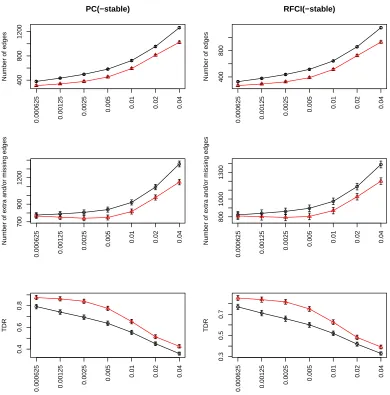
Figure 5 shows the number of edges, the number of errors, and the true discovery rate for the estimated skeletons, when compared to the true CPDAG or true PAG. The figure only compares PC and PC-stable in the setting without latent variables, and RFCI and RFCI-stable in the setting with latent variables, since the modifications for the v-structures and the orientation rules do not affect the estimation of the skeleton.
We first consider the number of estimated errors in the skeleton, shown in the first row of Figure 5. We see that PC-stable and RFCI-stable return estimated skeletons with fewer
edges than PC and RFCI, for all values of α. This can be explained by the fact that
PC-stable and RFCI-PC-stable tend to perform more tests than PC and RFCI (see also Appendix
A.2). Moreover, for all algorithms smaller values ofα lead to sparser outputs, as expected.
When interpreting these plots, it is useful to know that the average number of edges in the true CPDAGs and PAGs is about 1000. Thus, for all algorithms and almost all values of
α, the estimated graphs are too sparse.
The second row of Figure 5 shows that PC-stable and RFCI-stable make fewer errors
in the estimation of the skeletons than PC and RFCI, for all values of α. This may be
somewhat surprising given the observations above: for most values of α the output of PC
and RFCI is too sparse, and the output of PC-stable and RFCI-stable is even sparser. Thus, it must be that PC-stable and RFCI-stable yield a large decrease in the number of false positive edges that outweighs any increase in false negative edges.
This conclusion is also supported by the last row of Figure 5, which shows that PC-stable
and RFCI-stable have a better True Discovery Rate (TDR) for all values of α, where the
TDR is defined as the proportion of edges in the estimated skeleton that are also present in the true skeleton.
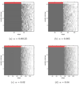
Figure 6 shows more detailed results for the estimated skeletons of PC and PC-stable
for one of the 250 graphs (randomly chosen), for four different values ofα. For each value of
α shown, PC yielded a certain number of stable edges that were present for all 20 variable
orderings, but also a large number of extra edges that seem to pop in or out randomly for different orderings. The PC-stable algorithm yielded far fewer edges (shown in red), and roughly captured the edges that were stable among the different variable orderings for PC. The results for RFCI and RFCI-stable show an equivalent picture.
5.3 Estimation of the CPDAGs and PAGs
We now consider estimation of the CPDAG or PAG, that is, also taking into account the edge orientations. For CPDAGs, we summarize the number of estimation errors using the Structural Hamming Distance (SHD), which is defined as the minimum number of edge insertions, deletions, and flips that are needed in order to transform the estimated graph into the true one. For PAGs, we summarize the number of estimation errors by counting the number of errors in the edge marks, which we call “SHD edge marks”. For example, if
● ● ● ● ● ● ● 400 800 1200 PC(−stable)
Number of edges
0.000625 0.00125
0.0025 0.005
0.01 0.02 0.04
● ● ● ● ● ● ● 400 800 RFCI(−stable)
Number of edges
0.000625 0.00125
0.0025 0.005
0.01 0.02 0.04
● ● ● ● ● ● ● 700 900 1200
Number of e
xtr
a and/or missing edges
0.000625 0.00125
0.0025 0.005
0.01 0.02 0.04
● ● ● ● ● ● ● 800 1000 1300
Number of e
xtr
a and/or missing edges
0.000625 0.00125
0.0025 0.005
0.01 0.02 0.04
● ● ● ● ● ● ● 0.4 0.6 0.8 TDR 0.000625 0.00125 0.0025 0.005
0.01 0.02 0.04
● ● ● ● ● ● ● 0.3 0.5 0.7 TDR 0.000625 0.00125 0.0025 0.005
0.01 0.02 0.04
Figure 5: Estimation performance of PC (circles; black line) and PC-stable (triangles; red line) for the skeleton of the CPDAGs (first column of plots), and of RFCI (circles; black line) and RFCI-stable (triangles; red line) for the skeleton of the PAGs
(second column of plots), for different values ofα (x-axis displayed in log scale).
edges
v
ar
iab
le order
ings
5 10 15 20
200 400
(a)α= 0.00125
edges
v
ar
iab
le order
ings
5 10 15 20
200 400 600 800
(b) α= 0.005
edges
v
ar
iab
le order
ings
5 10 15 20
200 400 600 800 1000 1200
(c)α= 0.02
edges
v
ar
iab
le order
ings
5 10 15 20
250 500 750 1000 1250 1500
(d) α= 0.04
Figure 6: Estimated edges with the PC-algorithm (black) for 20 random orderings on the variables, as well as with the PC-stable algorithm (red, shown as variable ordering 21), for a random graph from the high-dimensional setting. The edges along the
x-axes are ordered according to their presence in the 20 random orderings using
the original PC-algorithm. Edges that did not occur for any of the orderings were omitted.
then that counts as one error, while it counts as two errors if the true PAG contains, for
example, Xi ←Xj orXi and Xj are not adjacent.
Figure 7 shows that the PC-stable and RFCI-stable versions have significantly better
estimation performance than the versions with the original skeleton, for all values of α.
Moreover, MPC(-stable) and CPC(-stable) perform better than PC(-stable), as do MRFCI(-stable) and CRFCI(-MRFCI(-stable) with respect to RFCI(-MRFCI(-stable). Finally, for PC the idea to introduce bi-directed edges and lists in LCPC(-stable) and LMPC(-stable) seems to make little difference.
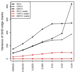
Figure 8 shows the variance in SHD for the CPDAGs, see Figure 8(a), and the variance in SHD edge marks for the PAGs, see Figure 8(b), both computed over the 20 random variable orderings per graph, and then plotted as averages over the 250 randomly
gener-ated graphs for the different values of α. The PC-stable and RFCI-stable versions yield
More-over, the variance is further reduced for (L)CPC-stable and (L)MPC-stable, as well as for CRFCI-stable and MRFCI-stable, as expected.
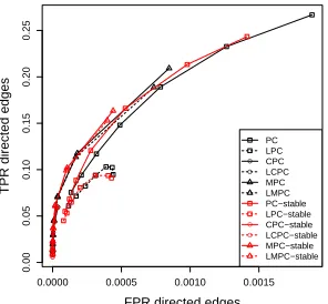
Figure 9 shows receiver operating characteristic curves (ROC) for the directed edges in the estimated CPDAGs (Figure 9(a)) and PAGs (Figure 9(b)). We see that finding directed edges is much harder in settings that allow for hidden variables, as shown by the lower true positive rates (TPR) and higher false positive rates (FPR) in Figure 9(b). Within each figure, the different versions of the algorithms perform roughly similar, and MPC-stable and MRFCI-stable yield the best ROC-curves.
1000 1200 1400 1600 SHD 0.000625 0.00125 0.0025 0.005
0.01 0.02 0.04 ● ● ● ● ● ● ● ● ● ● ● ● ● ● ● ● ● ● ● ● ● ● ● ● ● ● ● ● ● ● ● ● PC LPC CPC LCPC MPC LMPC PC−stable LPC−stable CPC−stable LCPC−stable MPC−stable LMPC−stable
(a) Estimation performance of (L)PC(-stable), (L)CPC(-stable), and (L)MPC(-stable) for the CPDAGs in terms of SHD.
2000
2500
3000
3500
SHD edge mar
ks
0.000625 0.00125
0.0025 0.005
0.01 0.02 0.04
● ● ● ● ● ● ● ● ● ● ● ● ● ● ● ● RFCI CRFCI MRFCI RFCI−stable CRFCI−stable MRFCI−stable
(b) Estimation performance of RFCI(-stable), CRFCI(-stable), and MRFCI(-stable) for the PAGs in terms of SHD edge marks.
Figure 7: Estimation performance in terms of SHD for the CPDAGs and SHD edge marks for the PAGs, shown as averages over 250 randomly generated graphs and 20
random variable orderings per graph, for different values of α (x-axis displayed
in log scale).
6. Yeast Gene Expression Data
We also compared the PC and PC-stable algorithms on the yeast gene expression data
(Hughes et al., 2000) that were already briefly discussed in Section 1. We recall that
we chose these data since they contain both observational and experimental data, obtained under similar conditions. The observational data consist of gene expression measurements of
5361 genes for 63 wild-type cultures (observational data of size 63×5361). The experimental
data consist of gene expression measurements of the same 5361 genes for 234 single-gene
0 50 100 150 V ar
iance of SHD
0.000625 0.00125
0.0025 0.005
0.01 0.02 0.04
● ● ● ● ● ● ● ● ● ● ● ● ● ● ● ● ● ● ● ● ● ● ● ● ● ● ● ● ● ● ● ● PC LPC CPC LCPC MPC LMPC PC−stable LPC−stable CPC−stable LCPC−stable MPC−stable LMPC−stable
(a) Estimation performance of (L)PC(-stable), (L)CPC(-(L)PC(-stable), and (L)MPC(-stable) for the CPDAGs in terms of the vari-ance of SHD.
0 200 400 600 800 V ar
iance of SHD edge mar
ks
0.000625 0.00125
0.0025 0.005
0.01 0.02 0.04
● ● ● ● ● ● ● ● ● ● ● ● ● ● ● ● RFCI CRFCI MRFCI RFCI−stable CRFCI−stable MRFCI−stable
(b) Estimation performance of
RFCI(-stable), CRFCI(-stable), and
MRFCI(-stable) for the PAGs in terms of the vari-ance SHD edge marks.
Figure 8: Estimation performance in terms of the variance of the SHD for the CPDAGs and SHD edge marks for the PAGs over the 20 random variable orderings per graph,
shown as averages over 250 randomly generated graphs, for different values ofα
(x-axis displayed in log scale).
In Section 6.1 we consider estimation of the skeleton of the CPDAG, and in Section 6.2 we consider estimation of bounds on causal effects. We used the same data pre-processing as in Maathuis et al. (2010).
6.1 Estimation of the Skeleton
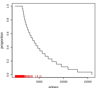
We applied PC and PC-stable to the (pre-processed) observational data. We saw in Section 1 that the PC-algorithm yielded estimated skeletons that were highly dependent on the variable ordering, as shown in black in Figure 10 for the 26 variable orderings (the original ordering and 25 random orderings of the variables). The PC-stable algorithm does not suffer from this order-dependence, and consequently all these 26 random orderings over the variables produce the same skeleton which is shown in the figure in red. We see that the PC-stable algorithm yielded a far sparser skeleton (2086 edges for PC-PC-stable versus 5015-5159 edges for the PC-algorithm, depending on the variable ordering). Just as in the simulations in Section 5 the order-independent skeleton from the PC-stable algorithm roughly captured the edges that were stable among the different order-dependent skeletons estimated from different variable orderings for the original PC-algorithm.
0.0000 0.0005 0.0010 0.0015 0.00 0.05 0.10 0.15 0.20 0.25
FPR directed edges
TPR directed edges
● ● ● ● ● ● ● ● ● ● ● ● ● ● ● ● ● ● ● ● ● ● ● ● ● ● ● ● ● ● ● ● PC LPC CPC LCPC MPC LMPC PC−stable LPC−stable CPC−stable LCPC−stable MPC−stable LMPC−stable
(a) Estimation performance of (L)PC(-stable), (L)CPC(-(L)PC(-stable), and (L)MPC(-stable) for the CPDAGs in terms of TPR and FPR for the directed edges.
0.0 0.1 0.2 0.3 0.4 0.5 0.6
0.000 0.005 0.010 0.015 0.020 0.025
FPR directed edges
TPR directed edges
● ● ● ●●● ● ● ● ● ●●● ● ● ● RFCI CRFCI MRFCI RFCI−stable CRFCI−stable MRFCI−stable
(b) Estimation performance of
RFCI(-stable), CRFCI(-stable), and
MRFCI(-stable) for the PAGs in terms of TPR and FPR for the directed edges.
Figure 9: Estimation performance in terms of TPR and FPR for the directed edges in CPDAGs and PAGs, shown as averages over 250 randomly generated graphs and 20 random variable orderings per graph, where every curve is plotted with respect
to the different values ofα.
PC-algorithm. Set 1 contained 1478 edges (7 directed edges), while Set 2 contained 1700 edges (20 directed edges).
Table 3 shows how well the PC and PC-stable algorithms could find these stable edges in terms of number of edges in the estimated graphs that are present in Sets 1 and 2 (IN), and the number of edges in the estimated graphs that are not present in Sets 1 and 2 (OUT). We see that the number of estimated edges present in Sets 1 and 2 is about the same for both algorithms, while the output of the PC-stable algorithm has far fewer edges which are not present in the two specified sets.
Throughout our analyses of the yeast data, we used tuning parameter α = 0.01, as
in Maathuis et al. (2010). We are not aware of any fully satisfactory method to choose
α in practice. In Appendix B, we briefly mention two possibilities that were described in
Maathuis et al. (2009): optimizing a Bayesian Information Criterion (BIC) and stability
selection (Meinshausen and B¨uhlmann, 2010).
6.2 Estimation of Causal Effects
edges
v
ar
iab
le order
ings
5 10 15 20 25
5000 10000 15000
(a) As Figure 1(a), plus the edges occur-ring in the unique estimated skeleton using the PC-stable algorithm over the same 26 variable orderings (red, shown as variable ordering 27).
0.0
0.2
0.4
0.6
0.8
1.0
edges
propor
tion
5000 10000 15000
(b) The step function shows the propor-tion of the 26 variable orderings in which the edges were present for the original PC-algorithm, where the edges are ordered as in Figure 10(a). The red bars show the edges present in the estimated skeleton using the PC-stable algorithm.
Figure 10: Analysis of estimated skeletons of the CPDAGs for the yeast gene expression data (Hughes et al., 2000), using the PC and PC-stable algorithms with tuning
parameter α = 0.01. The PC-stable algorithm yields an order-independent
skeleton that roughly captures the edges that were stable among the different variable orderings for the original PC-algorithm.
Edges Directed edges
PC PC-stable PC PC-stable
Set 1 IN 1478 (0) 1478 (0) 7 (0) 7 (0)
OUT 3606 (38) 607 (0) 4786 (47) 1433 (7)
Set 2 IN 1688 (3) 1688 (0) 19 (1) 20 (0)
OUT 3396 (39) 397 (0) 4774 (47) 1420 (7)
Figure 1(b) showed that IDA with the original PC-algorithm is highly order-dependent. Figure 11 shows the same analysis with PC-stable (solid black lines). We see that using PC-stable generally yielded better and more stable results than the original PC-algorithm. Note that some of the curves for PC-stable are worse than the reference curve of Maathuis et al. (2010) towards the beginning of the curves. This can be explained by the fact that the original variable ordering seems to be especially “lucky” for this part of the curve (see Figure 1(b)). There is still variability in the ROC curves in Figure 11 due to the order-dependent v-structures (because of order-order-dependent separating sets) and orientations in the PC-stable algorithm, but this variability is less prominent than in Figure 1(b). Finally, we see that there are 3 curves that produce a very poor fit.
False positives
0 1000 2000 3000 4000
0 200 400 600 800 1000 1200 1400 1600 1800 2000 2200 2400
T
rue positiv
es
Figure 11: ROC curves corresponding to the 25 random orderings of the variables for the analysis of yeast gene expression data (Hughes et al., 2000), where the curves are generated as in Maathuis et al. (2010) but using PC-stable (solid black lines)
and MPC-stable and CPC-stable (dashed black lines) withα= 0.01. The ROC
curves from Maathuis et al. (2010) (dashed blue) and the one for random guessing (dashed-dotted red) are shown as references. The resulting causal rankings are less order-dependent.
False positives
0 2000 4000 6000 8000 10000 0
2000 4000 6000 8000
T
rue positiv
es
MPC−stable RG PC
PC−stable
PC + SS MPC−stable + SS(P) PC + SSP
PC−stable + SSP PC−stable + SS
Figure 12: Analysis of the yeast gene expression data (Hughes et al., 2000) for PC, PC-stable, and MPC-stable algorithms using the original ordering over the variables (solid lines), using 100 runs stability selection without permuting the variable orderings, labelled as + SS (dashed lines), and using 100 runs stability selection with permuting the variable orderings, labelled as + SSP (dotted lines). The grey line labelled as RG represents the random guessing.
Another possible solution for the order-dependence orientation issues would be to use
stability selection (Meinshausen and B¨uhlmann, 2010) to find the most stable orientations
among the runs. In fact, Stekhoven et al. (2012) already proposed a combination of IDA and stability selection which led to improved performance when compared to IDA alone, but they used the original PC-algorithm and did not permute the variable ordering. We present here a more extensive analysis, where we consider the PC-algorithm (black lines), the PC-stable algorithm (red lines), and the MPC-stable algorithm (blue lines). Moreover, for each one of these algorithms we propose three different methods to estimate the CPDAGs and the causal effects: (1) use the original ordering of the variables (solid lines); (2) use the same methodology used in Stekhoven et al. (2012) with 100 stability selection runs but without permuting the variable orderings (labelled as + SS; dashed lines); and (3) use the same methodology used in Stekhoven et al. (2012) with 100 stability selection runs but permuting the variable orderings in each run (labelled as + SSP; dotted lines). The results are shown in Figure 12 where we investigate the performance for the top 20000 effects instead of the 5000 as in Figures 1(b) and 11.