Published online December 31, 2014 (http://www.sciencepublishinggroup.com/j/acm) doi: 10.11648/j.acm.20140306.18
ISSN: 2328-5605 (Print); ISSN: 2328-5613 (Online)
The Taylor Vortex and the driven cavity problems in the
stream function-Vorticity formulation
Blanca Bermúdez Juárez
1, *, René Posadas Hernández
2, Wuiyevaldo Fermín Guerrero Sánchez
21
Faculty of Computer Science, Autonomous University of Puebla (BUAP), Puebla, México 2
Faculty of Physics and Mathematics, Autonomous University of Puebla (BUAP), Puebla, México
Email address:
[email protected] (B. B. Juárez)
To cite this article:
Blanca Bermúdez Juárez, René Posadas Hernández, Wuiyevaldo Fermín Guerrero Sánchez. The Taylor Vortex and the Driven Cavity Problems in the Stream Function-Vorticity Formulation. Applied and Computational Mathematics. Vol. 3, No. 6, 2014, pp. 337-342.
doi: 10.11648/j.acm.20140306.18
Abstract:
In this work, two problems will be presented: The Taylor Vortex problem and the Driven Cavity problem. Both problems are solved using the Stream function-Vorticity formulation of the Navier-Stokes equations in 2D. Results are obtained using two methods: A fixed point iterative method and another one working with matrixes A and B resulting from the discretization of the Laplacian and the advective term, respectively. This second method resulted faster than the fixed point iterative one.Keywords:
Taylor Vortex Problem, Driven Cavity Problem, Navier-Stokes Equations, Stream Funtion-Vorticity Formulation1. Introduction
In this work results for the Taylor Vortex problem and the driven cavity problem will be presented. The formulation used is the Stream Function-Vorticity formulation of the Navier-Stokes equations in 2D. The equations are solved using finite differences and two methods: a fixed point iterative method and another one working with both matrixes A and B resulting from the discretization of the Laplacian and the advective term, respectively. The iterative method has already been used for solving the Navier-Stokes and Boussinesq equations in different formulations, [3 - 6].
With the fixed point iterative method used in [1], the idea was to work with a symmetric positive definite matrix. This scheme worked very well, as shown in [3 - 7], but the processing time, was in general, very large, especially for high Reynolds numbers. With the second method we are working with a matrix which is not symmetric, but it can be proved that it is strictly diagonally dominant for ∆t sufficiently small. The processing time was more or less 30% to 35% smaller when using this method.
2. Mathematical Model
Let D = Ω × (0, ), T > 0, Ω ⊂ , be the region of the flow of an unsteady isothermal incompressible fluid and Г its
boundary. These flows are governed by the non-dimensional system of equations in D, defined by:
u − ∇ u + ∇p + u ∙ ∇u = f (1) ∇ ∙ u = 0 (2) These are the Navier-Stokes equations in primitive variables, where u is the velocity, p is the pressure and the dimensionless parameter Re is the Reynolds number. This system must be supplemented with appropriate initial and boundary conditions: ( , 0) = ( ) in Ω and = on Г, respectively. In order to avoid the pressure variable and the incompressibility condition in Eq. (2), the Stream function-Vorticity formulation is used here.
The Stream function ψ is defined by:
= , = ! (3)
where u and v are the velocities in x and y-axis, respectively. In this case,(u ∙ ∇)ψ = 0. The vorticity is defined as the curl of the velocity field, and in 2D it is defined as:
# = $− %! (4)
# − ∇ # + u ∙ ∇# = 0 (5) ∇ ψ = −# (6) These are the Navier-Stokes equations in the Stream function-Vorticity formulation.
3. The Numerical Method
We approximate the time derivative by the second-order scheme:
# ( , (& + 1)∆)) ≈+,-./01,∆-2,-3/ (7)
where & ≥ 1, ∈Ω and ∆) > 0 is the time step.
At each time level the following nonlinear system defined in Ω has to be solved:
∇ ψ = −#, ψ|Г= 0 (8a)
αω − ∇ # + u ∙ ∇# = ;<, ω|Г= ω=> (8b)
where ∝= +
∆, and ;<=1,
-0,-3/
∆ . In the first time step, to
obtain (ψ , # ), any second order strategy using a combination of one step can be applied. Eq. (8b) is a transport type equation.
To solve Eq. (8a)-(8b) two strategies were used in this work: First we used a fixed point iterative method, described in [1].
Denoting
,(#, ψ) = αω − ∇ # + u ∙ ∇# − ;< (9)
system (8a)-(8b) is equivalent to:
∇ ψ = −#, ψ|Г= 0 (10a)
,(#, ψ) = 0, ω|Г= ω=> (10b)
So then Eq. (10a)-(10b), at time level n+1, are solved via the following iterative process [1]:
Given # = #@, and ψ = ψ@, solve until convergence in ω and Ψ:
∇ ψA2 = −#A, in Ω, ψA2 |
Г= 0 (11a)
BCD − ∇ E #A2 = #AF
,(#A, ψA2 ), in Ω (11b)
#A2 = # =>
A2 on Г, ρ>0;
and then take
(#@2 , ψ@2 ) = (#A2 , ψA2 ).
In order to reduce computing time we worked on solving Eq. (8a)-(8b) by the following method at each time step:
∇ ψ@2 = −#@ (12a)
BCD −HGIJE #@2 + HK#@2 = ;< (12b)
where = . Then, equation (12b) is solved using Gauss-Seidel.
4. Numerical Experiments
With respect to the driven cavity problem, Ω=(0,1)×(0,1). The top wall is moving with a nonzero velocity given by (1,0) and for the other three walls the velocity is given by (0,0). Following Goyon [17] ψ=0 is chosen on Г. As already
mentioned, ψ is overdetermined on the boundary (
@|Г is
also known) and no boundary condition is given for #. Several alternatives have been proposed, we follow the alternative given by Goyon [8]. A translation of the boundary condition in terms of the velocity (primitive variable) has to be used. By Taylor expansion of (8a) on the boundary for the driven cavity the following boundary conditions for ω are
obtained:
(
)
(
) (
)
( )
22
1
0, , 8ψ , , ψ 2 , ,
2
= − x − x + x
x
y t h y t h y t O h
h
ω (13a)
(
)
(
) (
)
( )
22
1
, , 8ψ , , ψ 2 , ,
2 x x x x
a y t a h y t a h y t O h h
ω = − − − − + (13b)
(
)
(
) (
)
( )
22
1
, 0, 8ψ , , ψ , 2 ,
2 y y y y
x t x h t x h t O h
h
ω = − − +
(13c)
#
(
)
(
) (
)
( )
22
1 3
, , 8ψ , , ψ , ,
2 y y y y y
x b t x b h t x b h t O h h h
= − − − − − + (13d)
with ℎ!, ℎ space steps.
(a) (b)
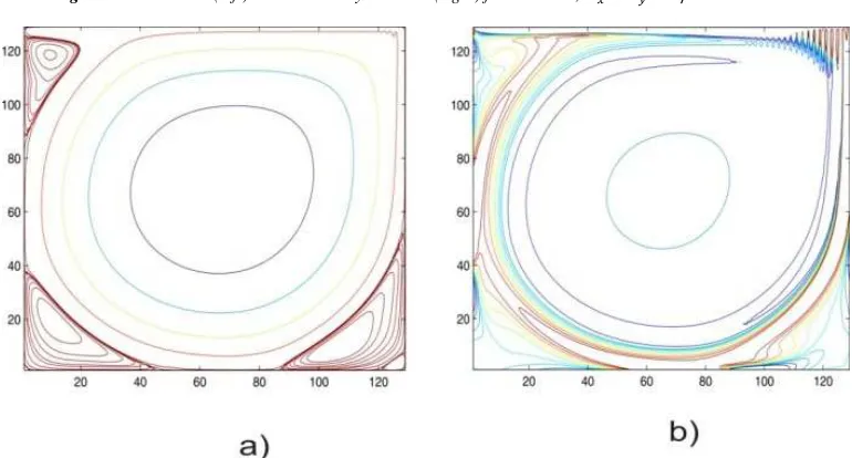
Figure 1. Streamlines (left) and isovorticity contours (right) for Re=5000, ℎ!= ℎ = 1/64 and t=100.
Figure 2. Streamlines (left) and isovorticity contours (right) for Re=7500, ℎ!= ℎ = 1/128 and t=100.
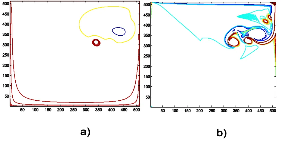
Figure 4. Streamlines (left) and isovorticity contours (right) for Re=31000, ℎ!= ℎ = 1/512 and t=5.
In Table 1 we show a table comparing the times for both methods: the Fixed Point Iterative Method (F.P.I. method) and the second one, working with both matrixes, A and B, resulting from the discretization of the Laplacian and the advective term respectively.
Table 1. Time (in seconds) for the Reynolds Numbers given and the two
methods described, for the Lid Driven Cavity problem.
Reynolds Number Hx=Hy F.P.I Method Using A And B
5000 1/64 612 480
7500 1/128 2441 3204
25000 1/768 61624 27402
31000 1/512 18864 10013
For the Taylor Vortex problem we show results for Re =5000 and Re=7500, withℎ = 1/64 , and t=10. For Re=5000 we show the exact stream function and vorticity.
For this problem, Ω = T0,2UV × T0,2UV. The exact solution is given by the following equations:
( , W, )) = − XYZ( ) [\&(W) \3I]^_ (14a)
( , W, )) = [\&( ) XYZ(W) \3I]^_ (14b)
In the primitive variable formulation we have, as initial conditions:
( , W, 0) = − XYZ( ) [\&(W) (15a) ( , W, 0) = [\&( ) XYZ(W) (15b) The stream function ` and vorticity#are defined by:
= ` , = −`!,# = − ! (16)
The initial conditions for the stream function and the
vorticity are obtained from equations (14) - (16):
`( , W, 0) = XYZ( )XYZ(W) (17) #( , W, 0) = −2 XYZ( ) XYZ(W) (18) The boundary conditions for the stream function and the vorticity are obtained from equations (14) and (16). For the stream function, these boundary conditions are:
ψ( , 0, )) = ψ( , 2U, )) = XYZ( )\3I]^_ (19a)
ψ(0, W, )) = ψ(2U, W, )) = XYZ(W)\3I]^_ (19b)
For the vorticity, the boundary conditions are:
ω( , 0, )) = ω( , 2U, )) = 2XYZ( )\3I]^_ (20a)
ω(0, W, )) = ω(2U, W, )) = 2XYZ(W)\3I]^_ (20b)
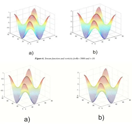
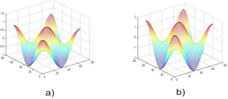
Next, in Figure 5 we show streamlines and isovorticity contours for Re=5000 and t=10 with h=2π/64. In Figure 6 we show the graphs of the stream function and the vorticity in 3-D for Re=5000 at t=10. In Figure 7 we show the exact solution for Re=5000 and t=10 and they look the same. In Figure 8 we show the streamlines and the isovorticity contours for Re=7500 and t=10 with h=2π/64, respectively. Again, with both methods, we get the same results. We show the graph in 3D of the stream function and vorticity in order to see the difference in scales at different times and for the different Reynolds numbers mentioned. In Table 2 we also show the times comparing the two methods.
Table 2. Time (in seconds) for the two Reynolds Numbers given and the two
methods described, for the Taylor Vortex problem.
Reynolds Number F.P.I Method Using A And B
5000 62 51
Figure 5. Streamlines and vorticity contours for Re=5000 and t=10.
Figure 6. Stream function and vorticity forRe=5000 and t=10.
Figure 8. Stream function and vorticity for Re=7500 and t=10.
5. Conclusions
For the driven cavity problem, results agree very well with those reported in the literature [3-6], [9,10] and with the second method, introduced here, we were able to reduce processing time for about 30% to 35%, for moderate Reynolds numbers and almost 50% for high Reynolds numbers. It can be seen in Figures 1 and 2, oscillations occur because the Reynolds number is very large, so it is necessary to use smaller values of h [13], numerically for stability and physically to capture the fast dynamics of the flow. For high Reynolds numbers and small values of h the computational work takes some days, so reducing the time is very important. For the Taylor vortex problem [7], [11], we were able to reduce processing time for about 20%.
We are still trying to reduce processing time. Till now we are using Fishpack [12] for solving equation (12a), which is an elliptic equation. We are working on solving this equation using Gauss-Seidel or SOR methods instead of using Fishpack, since the equation we are solving is a very simple one and Fishpack is used for solving a more general kind of equations.
References
[1] Nicolás A., A finite element approach to the Kuramoto-Sivashinski equation, Advances in Numerical Equations and Optimization, Siam (1991).
[2] Bermúdez B. and Juárez L., Numerical solution of an advection-diffusion equation, Información Tecnológica (2014) 25(1):151-160
[3] Bermúdez B., Nicolás A., Sánchez F. J., Buendía E., Operator Splitting and upwinding for the Navier-Stokes equations,
Computational Mechanics (1997) 20 (5): 474-477
[4] Nicolás A., Bermúdez B., 2D incompressible viscous flows at moderate and high Reynolds numbers, CMES (2004): 6(5): 441-451.
[5] Nicolás A., Bermúdez B., 2D Thermal/Isothermal incompressible viscous flows, International Journal for
Numerical Methods in Fluids (2005) 48: 349-366
[6] Bermúdez B., Nicolás A., Isothermal/Thermal Incompressible Viscous Fluid Flows with the Velocity-Vorticity Formulation,
Información Tecnológica (2010) 21(3): 39-49.
[7] Bermúdez B. and Nicolás A., The Taylor Vortex and the Driven Cavity Problems by the Velocity-Vorticity Formulation,
Procedings 7th International Conference on Heat Transfer, Fluid Mechanics and Thermodynamics (2010).
[8] Goyon, O., High-Reynolds numbers solutions of Navier-Stokes
equations using incremental unknowns, Comput. Methods Appl. Mech. Engrg. 130, (1996) pp. 319-335.
[9] Glowinski R., Finite Element methods for the numerical simulation of incompressible viscous flow. Introduction to the control of the Navier-Stokes equations, Lectures in Applied
Mathematics (1991), AMS, 28.
[10] Ghia U., Guia K. N. and Shin C. T., High-Re Solutions for Incompressible Flow Using the Navier-Stokes equations and a Multigrid Method, Journal of Computational Physics (1982): 48, 387-411.
[11] Anson D. K., Mullin T. & Cliffe K. A. A numerical and
experimental investigation of a new solution in the Taylor vortex problemJ. Fluid Mech, (1988) 475 – 487.
[12] Adams, J.; Swarztrauber, P; Sweet, R. 1980: FISHPACK: A
Package of Fortran Subprograms for the Solution of Separable Elliptic PDE`s, The National Center for Atmospheric Research,
Boulder, Colorado, USA, 1980.
[13] Nicolás-Carrizosa, A. and Bermúdez-Juárez, B., Onset of