Multi-Objective Markov Decision Processes
for Data-Driven Decision Support
Daniel J. Lizotte [email protected]
Department of Computer Science, Department of Epidemiology & Biostatistics The University of Western Ontario
1151 Richmond Street London, ON N6A 3K7 Canada
Eric B. Laber [email protected]
Department of Statistics
North Carolina State University Raliegh, NC 27695
USA
Editor:Benjamin M. Marlin, C. David Page, and Suchi Saria
Abstract
We present new methodology based on Multi-Objective Markov Decision Processes for developing sequential decision support systems from data. Our approach uses sequential decision-making data to provide support that is useful to many different decision-makers, each with different, potentially time-varying preference. To accomplish this, we develop an extension of fitted-Qiteration for multiple objectives that computes policies for all scalar-ization functions, i.e. preference functions, simultaneously from continuous-state, finite-horizon data. We identify and address several conceptual and computational challenges along the way, and we introduce a new solution concept that is appropriate when different actions have similar expected outcomes. Finally, we demonstrate an application of our method using data from the Clinical Antipsychotic Trials of Intervention Effectiveness and show that our approach offers decision-makers increased choice by a larger class of optimal policies.
Keywords: multi-objective optimization, reinforcement learning, Markov decision pro-cesses, clinical decision support, evidence-based medicine
1. Introduction
tutoring systems (Brunskill and Russell, 2011), and water reservoir control (Castelletti et al., 2010). Although headway has been made in these application areas, progress is hampered by the fact that many sequential decisionsupportproblems are not modelled well by MDPs. One reason for this is that in most cases, human action selection is driven by multiple competing objectives; for example, a medical decision will be based not only on the effec-tiveness of a treatment, but also on its potential side-effects, cost, and other considerations. Because the relative importance of these objectives varies from user to user, the quality of a policy is not well captured by a universal single scalar “reward” or “value.” Multi-Objective Markov Decision Processes (MOMDPs) accommodate this by allowing vector-valued re-wards (Roijers et al., 2013) and proposing an application-dependent solution concept. A solution concept is essentially a partial order on policies; the set of policies that are maxi-mal according to the partial order are considered “optimaxi-mal” and are indistinguishable under that solution concept. Depending on the application, a single policy may be selected from among these, or a set of policies may be presented in some way. Computing and presenting a set of policies is termed thedecision supportsetting by Roijers et al. and is the setting we consider here.
2. Existing Methods and Our Contributions
Roijers et al. (2013) note that, “...there are currently no methods for learning multiple poli-cies with non-linear [preferences] using a value-function approach.” We present a method that fills this gap, and that additionally uses value function approximation to accommo-date continuous state features, thus allowing us to use the MOMDP framework to analyze continuous-valued sequential data. Previous work (Lizotte et al., 2012) on this problem computes a set of policies based on the assumptions that i) end-users have a “true reward function” that is linear in the objectives and ii) all future actions will be chosen optimally with respect to the same “true reward function” over time. Our new method relaxes both of these assumptions as it allows the decision-maker to revisit action selection at each decision point in light of new information, both about state and about their own preferences and priorities over different outcomes of interest. Therefore, the proposed method can accom-modate changes in preference over time while still making optimal decisions according to our new solution concepts by introducing the non-deterministic multi-objective fitted-Q al-gorithm, which computes policies for all scalarization functions, i.e., preference functions, si-multaneously from continuous-state, finite-horizon data. This allows us to present a greater variety of action choices by acknowledging that preference functions may be non-linear. We then present the vector-valued expected returns associated with the different policies in order to provide decision support without having to refer to any particular scalarization function. Showing the expected returns in the original reward space allows us to more easily understand the qualitative differences between action choices. Although decision support is important in many application areas, we are motivated by clinical decision-making; there-fore we demonstrate the use of our algorithm using data from the Clinical Antipsychotic Trials of Intervention Effectiveness (CATIE).
• We introduce a complete non-deterministic fitted-Q algorithm that is applicable to arbitrary numbers of actions and arbitrary time horizons. (Previous work was limited to binary actions and maximum two decision points.) This allows us to perform fitted-Q backups in general settings using multiple reward functions over continuous-valued state features.
• We prove that our algorithm finds all policies that are optimal for some scalarization function by considering a collection of policies at the next time step that is only polynomial in the data set size.
• We formalize a solution concept, practical domination, that is more flexible than Pareto domination for identifying whether an action is not desirable. A similar concept was introduced in previous work (Laber et al., 2014a), but we show that using practical domination, while useful, is problematic for more than two decision points because it is does not induce a partial order on actions. However, we show that a modification of practical domination leads to a partial ordering for any number of actions or time points.
• We demonstrate the use of our algorithm on the Clinical Antipsychotic Trials of Intervention Effectiveness (CATIE) and we compare our approach quantitatively and qualitatively with a competing approach derived from previous work of Lizotte et al. (2010, 2012).
3. Motivation
Our work is motivated by a clear opportunity for reinforcement learning methods to provide novel ways of analyzing data to produce high-quality, evidence-based decision support. We briefly review some specific applications here where we believe our approach could be particularly relevant.
3.1 Intelligent Tutorial Systems
Brunskill and Russell (2011), and Rafferty et al. (2011) study the automatic construction of adaptive pedagogical strategies for intelligent tutoring systems. They employ POMDP models to capture the partially observable and sequential aspect of this problem, using hidden state to represent a student’s knowledge. Their approach uses time taken to learn all skills as a cost, i.e., negative reward, that drives teaching action selection. Chi et al. (2011) use an MDP formulation and use “Normalized Learning Gain,” a quantification of skill acquisition, as a reward; however, they do not explicitly consider time spent. The ability to consider both of these rewards simultaneously would empower the learner or the teacher to emphasize one or the other over the course of their interaction with the system. The method we present could offer a selection of teaching actions that are all optimal for different preferences over these rewards, and possibly others as well.
3.2 Computational Sustainability
efficacy of several off-policy methods for developing control policies for mallard duck pop-ulations. Their output, rather than providing autonomous control, is intended to provide decision support for public environmental policy-makers. They use “number of birds har-vested per year” as the reward. However, in practical management plans, several outcomes may be of interest including minimum population size, program cost, and so on. Because formulating a (e.g. linear) trade-off among these rewards would be difficult, our method is relevant to this problem.
3.3 Treating Chronic Disease
Reinforcement learning has also been used as a means of analyzing sequential medical data to inform clinical decision-makers of the comparative effectiveness of different treatments (Shortreed et al., 2011). RL methods are suited to decision support for treating chronic illness where a good policyfor choosing treatments over time is crucial for success. Indeed, optimal policies—known as “Dynamic Treatment Regimes” in statistics and the behavioral sciences—have been learned for the management of chronic conditions including attention deficit hyperactivity disorder (Laber et al., 2014b), HIV infection (Moodie et al., 2007), and smoking addiction (Strecher et al., 2006). They have also been applied to sequences of diagnostics as well, for example in breast cancer (Burnside et al., 2012). We present a case study in this domain in Section 7.
4. Background
We introduce a new approach for solving Multi-Objective Markov Decision Processes with the goal of providing data-driven decision support. Our approach uses non-deterministic policies to encode the set of all non-dominated policies. In this section, we review the most relevant existing literature on MOMDPs and NDPs.
4.1 Multi-objective Optimization and MOMDPs
The most basic definition of a Markov Decision Process is as a 4-tuple xS,A, P, Ry where
S is a set of states, A is a set of actions, Pps, a, s1q “Prps1|s, aq gives the probability of a
state transition given action and current state, and Rps, aq is the immediate scalar reward obtained in state s when taking action a. One common goal of “solving” an MDP, if we assume a finite time horizon ofT steps, is to find a policy π :SÑA that maximizes
Vπpsq “Eπr T
ÿ
t“1
Rpst, atq|s1 “ss
pointwise for all states. In the preceding,Eπindicates that the expectation is taken assuming the state-action trajectories are obtained by following policyπ. Because in the finite-horizon setting that the optimal π is in general non-stationary (Bertsekas, 2007), we defineπ to be a sequence of functions πt fortP t1, ..., Tu, whereπt:StÑAt.
Like previous work by Lizotte et al. (2010, 2012) and by many others (Roijers et al., 2013), we focus on the setting where the definition of an MDP is augmented by assuming a D-dimensional reward vector Rpst, atq is observed at each time step. We define a
state transition functions Pt:StˆAtÑPpSt`1q wherePpSt`1q is the space of probability
measures on St`1, and reward functions Rt :StˆAt Ñ RD for tP t1, ..., Tu. In keeping with the Markov assumption, bothRt andPtdepend only on the current state and action.
In this work we assume finite action sets, but we donotassume that state spaces are finite. The valueof a policy π is then given by
Vπpsq “Eπr T
ÿ
t“1
Rtpst, atq|s1 “ss (1)
which is the expected sum of (vector-valued) rewards we achieve by following policy π. Just as “solving” an MDP is an optimization problem (i.e. we want the optimal value function or policy), “solving” a MOMDP is amulti-objective optimization(MOO) problem. Whereas in typical scalar optimization problems having a unique solution is viewed as typical or at least desirable, in the MOO setting, the most common goal is to produce aset
of solutions that are non-dominated.
Definition 1 (Non-dominated a.k.a. Pareto optimal solutions) Let X be the set of all feasible inputs to a multi-objective optimization problem with objectivefpxq. LetY be the range of f on X. (In the RL context, one can think of X as the set of all possible policies starting from a given state, and Y as their corresponding values, which are vectors in this case.) A solution vector yPY isnon-dominated if Ey1 PY s.t. @
iy1i ěyi and Diyi1 ąyi. A
preimage xPX of such a y is sometimes called an efficient solution, but we will also refer to such inputs as non-dominated.
A common goal in MOO is to find all of the non-dominated solutions (Miettinen, 1999; Ehrgott, 2005). Some work on MOMDPs has this same goal (Perny and Weng, 2010). One approach to finding non-dominated solutions of a MOO problem is to solve a set of optimization problems that are scalarizedversions of the MOO. A scalarization function ρ is chosen which maps vector-valued outcomes scalars and then one solves
max
xPX ρpfpxqq,
the scalar optimization defined by composing the vector-valued outcome function with the scalarization function. If a specific “correct” scalarization function is fixed and known, we can simply apply it to all outcome vectors and reduce our MOO problem to a scalar opti-mization problem (and arguably we never had a MOO problem to begin with.) Otherwise, we may seek solutions to scalarized problems for allρ belonging to some function class. We assume that any ρ of interest is non-decreasing along each dimension, that is, it is always preferable to increase a reward dimension, all else being equal. It is well-known (Miettinen, 1999) that the set of Pareto-optimal solutions corresponds to the set of all solutions that are optimal for some scalarization function; we will use these two views of optimality as we construct our algorithm.
Previous work by Lizotte et al. (2012) uses dynamic programming to compute policies for all possible scalar rewards that are a convex combination of the basis rewards, using Q-functions learned by linear regression. Thus the output produces the optimal policies for all ρ such that ρprq “ r|w, wd ą 0,
ř
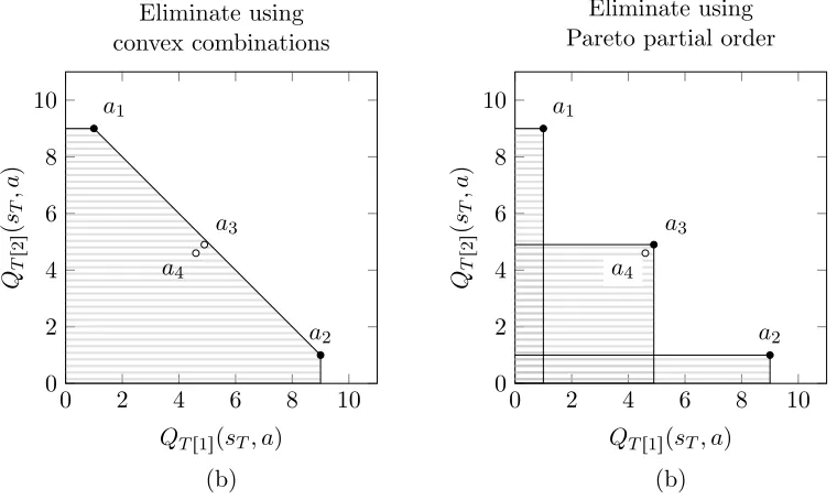
as a preference describing the relative importance of the the different basis rewards, and the method is used to show how preference relates to optimal action choice. This gives a new and potentially useful way of visualizing the connection between preference and action choice, but there are drawbacks to the approach. First, one must assume that the convex combination is fixed for all time points—that is, preferences do not change over time. This assumption enables dynamic programming to work, but is not reasonable for some applications, particularly in clinical decision-making where a patient’s first-hand experience with a treatment may influence subsequent preferences for symptom versus side-effect reduction. Second, the method is overly eager to eliminate actions. Consider two actions a1 and a2 that are extreme, e.g., a1 has excellent efficacy but terrible side-effects
and a2 has no side-effects but poor efficacy. These could eliminate a third actiona3 that is
moderately good according to both rewards. An example of this situation is illustrated in Figure 1 (a), which shows that the actions chosen by this method are restricted to the convex hull of the Pareto frontier, rather than the entire frontier. In this circumstance wherea3 is
qualitatively very different from both a1 and a2, we argue that a decision support system
should suggestall three treatments and thereby allow the decision-maker to make the final choice based on her expertise. The third drawback of using this approach is that it is limited to ordinary least squares regression, which may not work well for data with non-Gaussian errors, e.g., a binary terminal reward.
Rather than use the method of Lizotte et al., we will instead base our method on assessing actions and policies using a partial order on their vector of Q-values. Perhaps the most common partial order on vectors comes from the notion of Pareto-optimality
(Vamplew et al., 2011). For example, an action a is Pareto-optimal at a state sT if @pd, a1q Q
TrdspsT, aq ěQTrdspsT, a1q. We will show in Section 5 that fortăT, the problem
of deciding which actions are optimal is more complex, but we will still leverage the idea of a partial order. The problem of identifying Pareto-optimal policies is of significant interest in RL (Perny and Weng, 2010; Vamplew et al., 2009) and is closely related to what we wish to accomplish. Basing our work on the Pareto-optimal approach rather than on the previous work of Lizotte et al. avoids assuming that preferences are fixed over time, and it avoids the problem of “extreme” actions eliminating “moderate” ones. Furthermore, our approach works with a larger class of regression models, including ordinary least squares, the lasso, support vector regression, and logistic regression. While our Pareto-based approach makes these three improvements, using Pareto-optimality can still result actions being eliminated unnecessarily; this is illustrated in Figure 1(b). We address this problem by introducing an alternative notion of domination in Section 6. Each of these contributions leads to increased action choice for the decision-maker by considering a larger class of preferences over reward vectors.
4.2 Non-Deterministic Policies
0 2 4 6 8 10 0
2 4 6 8
10 a1
a3
a4
a2
QTr1spsT, aq pbq
QT
r
2
s
p
sT
,
a
q
Eliminate using convex combinations
0 2 4 6 8 10
0 2 4 6 8
10 a1
a3
a4
a2
QTr1spsT, aq pbq
QT
r
2
s
p
sT
,
a
q
Eliminate using Pareto partial order
Figure 1: Comparison of existing approaches to eliminating actions at time T. The prob-lems illustrated here have analogs for t ă T where the picture is more com-plicated. In this simple example, we suppose the vector-valued expected re-wardspQTr1spsT, aq, QTr2spsT, aqqarep1,9q, p9,1q, p4.9,4.9q, p4.6,4.6qfor actions
a1, a2, a3, a4, respectively. Figure 1(a): Using the method of Lizotte et al. (2010,
2012) based on convex combinations of rewards, actionsa3anda4would be
elimi-nated, and we would have ΠTpstq “ ta1, a2u. (Any action whose expected rewards
fall in the shaded region would be eliminated.) However, we would prefer to at least include a3 since it offers a more “moderate” outcome that may be
impor-tant to some decision-makers. Figure 1(b): Using the Pareto partial order, only action a4 is eliminated, and we have ΠTpsTq “ ta1, a2, a3u. However, we may
prefer to includea4 since its performance is very close to that ofa3, and may be
information.1 Given an MDP with state space S and an action set A, an NDP Π is a map from the state space to the set 2AztHu. Milani Fard and Pineau assume that a user
operating the MDP will, at each timestep, choose an action from the set Πpsq. They are motivated by the same considerations that we are in the sense that they wish to provide choice to the user while still achieving good performance; thus, they only eliminate actions that are clearly sub-optimal. Because they consider only a single reward function, they can measure performance using the expected discounted infinite sum of future (scalar) rewards in the usual way, and they can produce an NDP Π that has near-optimal performance even if the user chooses the “worst” actions from Πpsqin each state.
One can view the NDP as a compact way of expressing a set of policies that might be executed. Suppose that #A “ |Πpsq|, the number of actions provided by the NDP Π, is the same at all states. Then the number of policies that are consistent with Π, that is, the policies for which πpsq P Πpsq, is #A|S|. So the NDP Π is a compact encoding of an
exponential number of policies. We will make use of this property to encode our policies. The two most important differences between our work and that of Milani Fard and Pineau are that our motivation for learning non-deterministic policies is driven explicitly by having more than one basis reward of interest, and that we use more general value function models rather than a tabular representation. Having multiple basis rewards combined with value function approximation leads us to a different, novel algorithm for learning NDPs.
5. Fitted-Q for MOMDPs
Our non-deterministic fitted-Q algorithm for multiple objectives uses finite-horizon, batch data. We present a version that uses linear value function approximation because this model is commonly used by statisticians working in clinical decision support (Strecher et al., 2006; Lizotte et al., 2010, 2012; Laber et al., 2014b), and because available data often contain continuous-valued features, e.g., symptom and side-effect levels, laboratory values, etc., and outcomes, e.g., symptom scores, body mass index. It is a flexible model because we will not restrict the state features one might use. For learning, we assume a batch of n data trajectories of the form
si1, ai1, ri1r1s, ..., r1irDs, si2, ai2, ri2r1s, ..., r2irDs, ..., siT, aiT, rTir1s, ..., riTrDs fori“1, ..., n. In the following exposition, we begin by specifying how the algorithm works for the last time point t“T. This would be the only step needed in a “non-sequential” decision problem. We then describe the steps analogous to the fitted-Q “backup” operation for earlier timepointstăT, which are more complex.
5.1 Final time point, t“T
At timeT, we define the approximateQ-function for reward dimensiondas the linear least squares fit
ˆ
QTrdspsT, aTq “φTpsT, aTq|wˆTrds, wˆTrds “argmin w
ÿ
i
´
φTpsiT, aiTq
|
w´riTrds
¯2
(2)
giving the estimated vector-valued expected reward function
ˆ
QTpsT, aTq “ pQˆTr1spsT, aTq, ...,QˆTrDspsT, aTqq|. (3)
Here, φTpsT, aTq is a feature vector of state and action. As discussed by Lizotte et al.
(2012),φTpsT, aTqwould typically include: a constant component for the intercept, features
describing sT, dummy variables encoding the discrete action aT, and the product of the
dummy variables with the features describing sT (Cook and Weisberg, 1999). One could
also include other non-linear functions of sT and aT as features if desired. We present our
method assuming that ˆwTrdsare found by least squares regression, but one could for example add an L1 penalty, or use support vector regression (Hastie et al., 2001). Furthermore,
unlike previous work by Lizotte et al. (2012), any Generalized Linear Model (GLM) with a monotonic increasing link function (e.g. logistic regression, Poisson regression, and so on) can also be used (Cook and Weisberg, 1999). Note that we can recover a “tabular” representation if the states are discrete and we assign mutually orthogonal feature vectors to each one.
Having obtained the ˆQT from (2), we construct an NDP ΠT that will give, for each state,
the actions one might take at the last time point. For each statesT at the last time point,
each actionaT is associated with auniquevector-valued estimated expected reward given by
ˆ
QTpsT, aTq. Thus, we decide which among these vectors is a desirable outcome, and include
their associated actions in ΠTpsTq. Our main focus will be to construct ΠTpsTq for each
state based on the multi-objective criterion of Pareto optimality; however, an important advantage of our algorithm is that it can use other definitions of ΠT as well; we discuss an
extension in Section 6. For example, different definitions of ΠT allow us to recover other
varieties of Q-learning:
Scalar Fitted-Q: Defining
ΠTpsTq “ targ max a
ˆ
QTr0spsT, aqu
gives standard fitted-Qapplied to reward dimension 0.
Convex Pareto-optimal Fitted-Q: Defining
ΠTpsq “ ta:Dθ pθě0^θ|1“1^ @a1 QˆTpsT, aq|θ ěQˆTpsT, a1q|θqu
includes those actions whose expected reward is on the convex hull of the Pareto frontier; these are the actions that would be included by the previous method of Lizotte et al. (2012).
Pareto-optimal Fitted-Q: Defining
ΠTpsq “ ta:Ea1 p@dQˆTrdspsT, aq ăQˆTrdspsT, a1qqu
5.2 Earlier time points, tăT
For t ăT, it is only possible to define the expected return of taking an action in a given state by also deciding which particular policy will be followed to choose future actions. In standard fitted-Q, for example, one assumes that the future policy is given byπjpsq “
arg maxaQˆjps, aq for all j ą t. In the non-deterministic setting, we may know that the
future policy belongs to some set of possible policies derived from Πj for j ą t, but in
general we do not know which among that set will be chosen; therefore, we explicitly include the dependence of ˆQt on the choice of future policies πj, tăj ďT:
ˆ
Qtpst, at;πt`1, ..., πTq “
!
ˆ
Qtr1spst, at;πt`1, ..., πTq, ...,QˆtrDspst, at;πt`1, ..., πTq
)|
where
ford“1, . . . , D, Qˆtrdspst, at;πt`1, ..., πTq “φtpst, atq|wˆtrdsπt`1,...,πT, and
ˆ
wtrdsπt`1,...,πT“argmin
w n
ÿ
i“1
”
φtpsit, aitq
|
w´
!
ritrds`Qˆt`1rdsps i
t`1, πt`1psit`1q;πt`2, ..., πTq
)ı2
.
(4) We say an expected return is achievable if it can be obtained by taking some immediate action in the current state and following it with a fixed sequence of policies until we reach the last time point.
We use Qt to denote a set of partially-evaluated Q-functions; each member of Qt is a
function of st and at only and assumes a particular fixed sequence πt`1, ..., πT of future
policies. Precisely which future policies should be considered is the subject of the next section. For the last time point, we define QT “ tQˆTu, the set containing the single
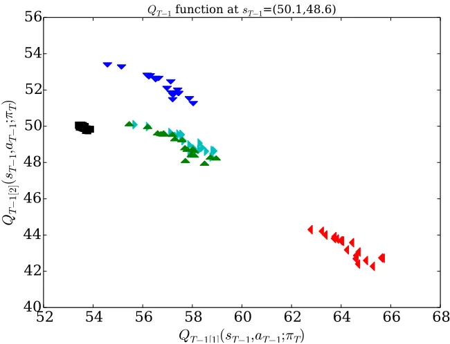
(multivariate) Q-function for the last time point. Figure 2 is a visualization of an example
QT´1 where each function in the set is evaluated at the same given state and for each of the five available actions,tİ,‚,IJ,§,đu. Thus, each element of the exampleQT´1corresponds to
a collection of five markers on the plot, one for the expected return for each action, assuming we follow a particularπT. The question of what collection of πT we should consider is the
subject of the next section.
5.3 Constructing Πt from Πt`1
We now describe the “backup” step that constructs Πt and Qt from Πt`1 and Qt`1. A
member of Qt is constructed from data using equation (4) by choosing two components:
An element of Qt`1 (with its implicit choice of πt`2 through πT) and a policyπt`1. When
considering different possibleπt`1, we restrict our attention to policies that i) areconsistent
with Πt`1, and ii) arerepresentableusing the approximation space chosen for ˆQt`1. In the
52
54
56
58
60
62
64
66
68
Q
T−1[1](
s
T−1,a
T−1;
π
T)
40
42
44
46
48
50
52
54
56
Q
T−1[
2]
(
s
T−1
,a
T−1
;
π
T)
Q
T−1function at
s
T−1=(50.1,48.6)
Figure 2: Partial visualization of the members of an example QT´1. We fix a statesT´1“
p50.1,48.6qin this example, and we plot ˆQT´1psT, aTqfor each ˆQT´1PQT´1 and
for eachaT´1 P tİ,‚,IJ,§,đu. For example, theİmarkers near the top of the plot
correspond to expected returns for each ˆQPQT that is achievable by taking the
İ action at the current time point and then following a particular future policy. This exampleQT´1 contains 20 ˆQT´1 functions, each assuming a differentπT.
Definition 2 (Policy consistency) A policy π is consistent with an NDP Π, denoted
π ĂΠ, if and only if πpsq PΠpsq @sPS. We denote the set of all policies consistent with
Π by CpΠq.
This restriction is analogous to fitted-Qin the scalar reward setting, where we estimate the current Q function assuming we will follow the greedy policy of the estimated optimal Q function at later time points. In our setting, there are likely to be multiple different policies whose values, pointwise at each state, are considered “optimal,” e.g. that are Pareto non-dominated. Although we cannot pare down the possible future policies to a single unique choice as in scalar fitted-Q, we can still make significant computational savings. Note that in the batch RL setting, two policies are distinguishable only if they differ in action choice on states observed in our data set. In the following, when we talk about the properties of policies, we mean in particular over the observed states in our data set. Where clarification is needed, we writeSn
t to mean then states observed in our data set at time t. Note that |CpΠtq| “ ˆstPSn
t|Πtpstq|, the product of the cardinalities of the sets produced by Πt over the observed data. Because|Πtpstq| ď |A|, we have|CpΠtq| ď |A|n. If Πtscreens out enough
0
25
State
50
75
100
1
2
Action
Non-deterministic policy
a1
a2
0
25
State
50
75
100
1
2
Action
Consistent policy
a1
a2
0
25
State
50
75
100
1
2
Action
Feature-consistent policy
a1
a2
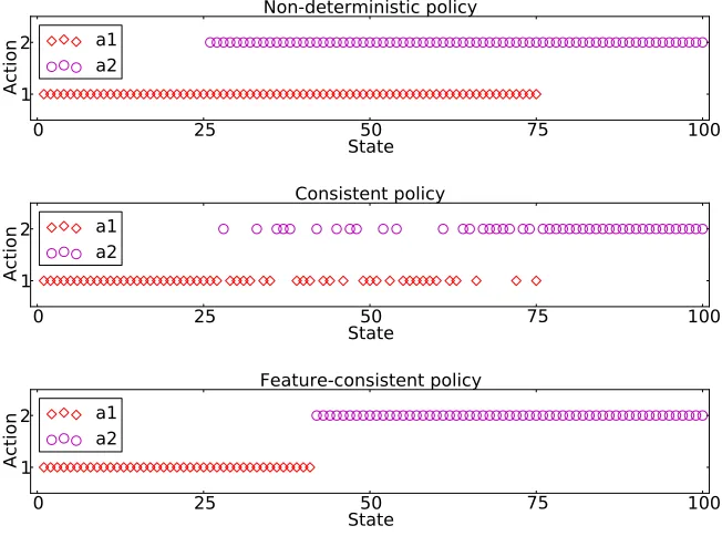
Figure 3: An NDP on a one-dimensional continuous state-space, a consistent policy, and a φ-consistent policy.
and if for some fraction η of the n trajectories (0 ăη ď 1) we have|Πtpstq| ě 2, then we
have |CpΠtq| PΩp2nq. Therefore in many interesting cases, computing a Qt that includes
even just the consistent future policies is computationally intractable.
We therefore impose a further restriction on possible future policies, again only elimi-nating policies we do not wish to consider. In scalar fitted-Q, the learned optimal policy is given by argmaxaQps, aq. If the learned Q-functions are linear in some feature space, then the learned optimal policy can be represented by a collection of linear separators that divide feature space into regions where different actions are chosen. This is true for any
scalar reward signal. Therefore, in the scalar reward case for a given feature space, any future policy that cannot be represented in this way will never considered when computing
ˆ
Qfor earlier timepoints no matter what the observed rewards are.
In NDP settings where dimφtpst, atq ! n, most of the policies that are consistent with
Πtpstq are not representable in the form πpstq “ argmaxaQtpst, aq, and therefore would
linear regression. We therefore will “prune away” these consistent but un-representable policies in order to reduce the size ofQtby introducing the notion of policy φ-consistency.
Definition 3 (Policy φ-consistency) Given a feature map φ : SˆA Ñ Rp, we say a
policyπt isφ-consistent with a non-deterministic policyΠt over a data set with n
trajecto-ries, if and only ifDwp@iP1, ..., n πtpsitq PΠtpsitq ^πtpsitq “argmaxaφpsit, aq|wq. We write
πtĂφΠt, and we denote the set of all policies that are φ-consistent withΠt by CφpΠtq.
A φ-consistent policy is an element of CpΠtq that is the argmax policy for some (scalar)
Q-function over the feature map φ. The form of such a policy is much like that of the function learned by a structured-output SVM (Tsochantaridis et al., 2005).
We now show that the number ofφ-optimal policies for any given time point is polyno-mial in the data set sizen.
Theorem 1 Given a data set of size n, a feature mapφ, and an action set A, there are at most Opndimpφq¨ |A|2 dimpφqq feature-consistent policies.
Proof The space ofφ-consistent policies is exactly analogous to the space of linear mul-ticlass predictors withφ as their feature map. We therefore port two results from learning theory to analyze the number of φ-consistent policies in terms of the dimension of φ, the size of the data setn, and the size of the action set. TheNatarajan dimension(Natarajan, 1989; Shalev-Shwartz and Ben-David, 2014) is an extension of VC-dimension to the multi-class setting. For a supervised learning data set of size n, kclasses, and a hypothesis class
H with Natarajan dimension NdimpHq, the number|Hn|of hypotheses restricted to the n
datapoints is subject to the following upper bound due to Natarajan (1989):
|Hn| ďnNdimpHq¨k2 NdimpHq. (5)
Furthermore, the hypothesis class given by
Hφ“ txÞÑargmax i
φpx, iq|w:wPRdimφu (6)
has Natarajan dimension NdimpHφq “ dimpφq (Shalev-Shwartz and Ben-David, 2014).
Combining Equations (5) and (6) and completes our proof.
Theorem 1 shows that for fixed |A| and dimpφq there are only polynomially many φ-consistent future policies, rather than a potentially exponential number of φ-consistent policies as a function ofn. Therefore, by considering onlyφ-consistent future policies, we can ensure that the size of QT´1 is polynomial in n. The restriction toφ-consistent policies applies to Q-functions based on Generalized Linear Models with monotonic increasing link functions (such as logistic regression) as well. Such models have output of the formgpφpst, aq|wqfor
monotonic increasing g. For these models, argmaxagpφpsi, aq|wq “argmaxaφpst, aq|w, so
all of our results and algorithms forφ-consistency immediately apply.
We now express CφpΠq in a way that allows us to enumerate it using a Mixed Inte-ger Program (MIP). To formulate the constraints describing CφpΠq, we take advantage of
indicator constraints, a mathematical programming formalism offered by modern solvers; e.g. the CPLEX optimization software package as of version 10.0, which was released in 2006 (CPLEX). Each indicator constraint is associated with a binary variable, and is only enforced when that variable takes the value 1. To construct the MIP, we introduce nˆ |A|
indicator variablesαi,jthat indicate whetherπpsiq “jor not. We then impose the following
constraints:
@iP1, . . . , n, jP1, . . . ,|A|, αi,j P t0,1u (7)
@iP1, . . . , n, ÿ
j
αi,j “1 (8)
@iP1, . . . , n,@jP1, . . . ,|A|, αi,j “1 ùñ @k‰j, pφpsi, jq ´φpsi, kqq|wě1. (9)
Constraints (7) ensure that the indicator variables for the actions are binary. Constraints (8) ensure that, for each example in our data set, exactly one action indicator variable is on. The indicator constraints in (9) ensure that if the indicator for action j is on for the ith example, then weights must satisfy j “argmaxaφpsi, aq|w. Note that the margin
condition (i.e., having the constraint be ě1 rather than ě0) avoids a degenerate solution withw“0.
The above constraints ensure that any feasibleαi,jdefine a policy that can be represented
as an argmax of linear functions over the given feature space. Imposing the additional constraint that the policy defined is consistent with a given NDP Π is now trivial:
@iP1, ..., n, ÿ
jPΠpsiq
αi,j“1. (10)
Constraints (10) ensure that the indicator that turns on for the ith example in the data must be one that indicates an action that belongs to the set Πpsiq.
Note that we have not specified an objective for this MIP: for the problem of generating φ-consistent policies, we are only interested in generating feasible solutions and interpreting the label variables as a potential future policy. Software such as CPLEX can enumerate all possible discrete feasible solutions to the constraints we have formulated. To do so, we give the constraints to the solver and ask for solutions given an objective that is identically zero. Note that if we instead minimized the quadratic objective}w}2 subject to these constraints, we would recover the consistent policy with the largest margin between action choices in the feature space. The output would be equivalent to exact transductive learning of a hard-margin multiclass SVM using the actions as class labels (Tsochantaridis et al., 2005). Given Qt, our final task is to define Πtpstqfor all st. WhileQT is a singleton, fortăT
this is not the case in general, and we must take this into account when defining Πtpstq. We
present two definitions for Πtpstqbased on a strict partial orderă. (For example ămay be
the Pareto partial order.)
Π@
ăpstq “ ta:@Qˆ PQt pEpa1 ‰a,Qˆ1 PQtq pQˆpst, aqăQˆ1pst, a1qqqu
Algorithm 1 Non-deterministic fitted-Q
Learn ˆQT “ pQˆTr1s, ...,QˆTrDsq, set QT “ tQˆTu
for t“T ´1, T ´2, ...,1 do for allsi
tin the data do
Generate ΠD
ăpsitqusing Qt`1
QtÐ H
for allπtPCφpΠDăqdo
for allQˆt`1 PQt`1 do
Learn pQˆtr1sp¨,¨, πt, ...q, ...,QˆtrDsp¨,¨, πt, ...qqusing ˆQt`1, add to Qt
Under Π@
ă, action a is included if for all fixed sequences of policies we might follow after choosing a, no other choice of current action and future policy is preferable according to ă. Π@
ă is appealing in cases where we wish to guard against a na¨ıve decision maker choosing poor sequences of future actions. For theQT´1 shown in Figure 2, we would have
Π@
ăpsT´1q “ tİ,đu. The ‚ action is obviously eliminated because any İ point dominates
every single ‚ point. The IJ and § actions eliminate each other: There are IJ points that are dominated by § points, and § points that are dominated by IJ points. Note that this illustrates how Π@
ăpstq could be empty: if our example only contained the § and IJactions, we would have Π@
ăpsT´1q “ H. In practice we find that Π@ă can be very restrictive; we therefore present ΠD
ă as an alternative. Under ΠDă, action a is included if there is at least
onefixed future policy for whichais not dominated by a value achievable by anotherpa1,Qˆ1 q
pair. Note that ΠD
ă Ě Π@ă, and that because the relation ˆQ ă Qˆ1 is a partial order on a finite set, there must exist at least one maximal element; therefore ΠD
ăpstq ‰ H. In the Figure 2 example, we have ΠD
ăpsT´1q “ tİ,đ,§,IJu; note that‚is not included because there
is always another action that can dominate it if we choose an appropriate future policy. In order to provide increased choice and to ensure we do not generate NDPs with empty action sets, we will use ΠD
ăin our complete non-deterministic multiple-reward fitted-Qalgorithm, but in our examples we will investigate the effect of choosing Π@
ă instead.
5.4 Time Complexity
Pseudocode is given in Algorithm 1. The time cost of Algorithm 1 is dominated by the construction of Qt, whose size may increase by a factor of Opn|A|dimφq at each timestep;
therefore in the worst case |Q1| is exponential in T. This can be mitigated somewhat by
0 2 4 6 0
2 4 6
a1
a2
a3
a4
QTr1spsT, aq pbq
QT
r
2
s
p
sT
,
a
q
Eliminate using Practical Domination
0 2 4 6
0 2 4 6
a1
a2
a3
a4
QTr1spsT, aq pbq
QT
r
2
s
p
sT
,
a
q
Eliminate using Strong Practical Domination
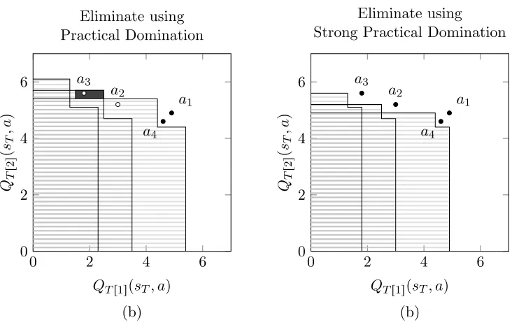
Figure 4: Comparison of rules for eliminating actions. In this simple example, we suppose theQ-vectorspQTr1spsT, aq, QTr2spsT, aqqarep4.9,4.9q,p3,5.2q,p1.8,5.6q,p4.6,4.6q
fora1, a2, a3, a4, respectively, and suppose ∆1 “∆2 “0.5. Figure 4(a): Using
the Practical Domination rule, actiona4 is not eliminated bya3 because it is not
much worse according to either basis reward, as judged by ∆1and ∆2. Actiona2is
eliminated because although it is slightly better thana1according to basis reward
2, it is much worse according to basis reward 1. Similarly,a3 is eliminated bya2.
Note the small solid rectangle to the left ofa2: points in this region (includinga3)
are dominated bya2, but not by a1. This illustrates the non-transitivity of the
Practical Domination relation, and in turn shows that it is not a partial order.
6. Practical domination
So far we have presented our algorithm assuming we will use Pareto dominance to defineă. However, there are two ways in which Pareto dominance does not reflect the reasoning of a physician when she determines whether one action is superior to another. First, an action that has a slightly lower value along a single dimension, but is otherwise equivalent, will be Pareto-dominated (and eliminated) even if this difference is clinically meaningless. A physician with this knowledge would consider both actions in light of other “tie-breaking” factors not known to the RL policy, e.g., cost, allergies, etc. Second, an action that is slightly better for one reward but much worse for another would not be dominated, even though it may realistically be a very poor choice, and perhaps even unethical. Chatterjee et al. (2006) introduced ε-dominance which would partially address the first issue, but not the second. We wish to eliminate only actions that are “obviously” inferior while maintaining as much freedom of choice as possible. To accomplish this, we use the idea of practical significance (Kirk, 1996) to develop a definition of domination based on the idea that in real-world applications, small enough differences in expected reward simply do not matter. Differences that fall below a threshold of importance are termed “practically insignificant.” We introduce two notions of domination that are modifications of Pareto domination. The first, Practical Domination, most accurately describes our intuition about the set of actions that should be recommended. However, we show that it has an undesirable non-transitivity property. We then describe an alternative strategy based on what we callStrong Practical Domination.
Definition 4 (Practical Domination) We say that an action a2 is practically
domi-nated by a1 at state sT, and we write a2 ăp a1, if both of the following hold
@dP1, . . . , D QtrdspsT, a2q ďQtrdspsT, a1q `∆d, (11) DdP1, . . . , D QtrdspsT, a2q ăQtrdspsT, a1q ´∆d. (12)
If either of the above do not hold, we write a2ćp a1.
Intuitively, an action a1 practically dominates a2 ifa2 is “not practically better” than
a1for any basis reward (property 11), and ifa2 is “practically worse” thana1 forsomebasis
reward (property 12). “Practically better” and “practically worse” are determined by the elicited differences ∆dě0. Note that we could have ∆ddepend on the current state if that
were appropriate for the application at hand; for simplicity we assume a uniform ∆d. We
might consider using the relationăpas the ordering that produces our NDP according to one
of the mappings from Section 5. Unfortunately, ăp is not transitive. Suppose that the
Q-vectorspQTr1spsT, aq, QTr2spsT, aqqarep4.9,4.9q,p3,5.2q,p1.8,5.6q,p4.6,4.6qfora1, a2, a3, a4,
respectively, and suppose ∆1 “∆2 “0.5. Then a2ăp a1 anda3 ăp a2 buta3ćp a1. This
non-transitivity causes undesirable behavior: if we consider only actions a1 and a3, we get
ΠD
ăpsTq “ ta1, a3u. However, if we consider a1, a2 and a3, we get ΠDăpsTq “ ta1u! Thus by consideringmore actions, we get asmallerΠD
ăpsTq. This is unacceptable in our domain, so we introduce an alternative.2
Definition 5 (Strong Practical Domination) We say an action a2 is strongly
practi-cally dominated by a1 at state sT, and we write a2ăsp a1, if both of the following hold.
@dP1, . . . , D QTrdspsT, a2q ďQTrdspsT, a1q (13)
DdP1, . . . , D QTrdspsT, a2q ăQTrdspsT, a1q ´∆d (14)
If either of the above do not hold, we write a2ćsp a1.
The relationăsp is transitive, and will not cause the unintuitive results ofăp. However, it
does not eliminate actions that are slightly better for one basis reward but much worse for another. (Note that DdP1...D, QTrdspsT, a2q ąQTrdspsT, a1q ùñ a2ćsp a1.) We propose
a compromise: we will use ăsp as our partial order for producing NDPs as in Section 5.
However, if an action a would have been eliminated according to ăp but not according to
ăsp, we may “warn” that it may be a bad choice. This has no impact on computation
of Π and ˆQ at earlier time points, but can warn the user that choosing a entails taking a practically significant loss on one basis reward to achieve a practicallyinsignificant gain on another.
7. Empirical Example: CATIE
We illustrate the output of non-deterministic fitted-Q using data from the Clinical An-tipsychotic Trials of Intervention Effectiveness (CATIE) study. The CATIE study was designed to compare sequences of antipsychotic drug treatments for the care of schizophre-nia patients. The full study design is quite complex (Stroup and al, 2003; Swartz et al., 2003); we use a simplified subset of the CATIE data in order to more clearly illustrate the proposed methodology. CATIE was an 18-month study of n “ 1460 patients that was divided into two main phases of treatment. Upon entry, most patients began “Phase 1,” and were randomized to one of five treatments3 with equal probability: olanzapineđ, risperidone§, quetiapineIJ, ziprasidoneİ, or perphenazine‚. As time passed, patients were given the opportunity to discontinue their Phase 1 treatment and begin “Phase 2” on a new treatment. The possible Phase 2 treatments depended on the reason for discontinu-ing Phase 1 treatment. If the Phase 1 treatment was ineffective at reducdiscontinu-ing symptoms, then patients entered the “Efficacy” arm of Phase 2, and their Phase 2 treatment was chosen randomly as: {clozapine˛} with probability 1{2, or uniformly randomly from the set {olanzapineđ, risperidone§, quetiapineIJ} with probability 1{2. Because relatively few patients entered this arm, and because of the uneven action probabilities, it is reasonable to combine {olanzapineđ, risperidone§, quetiapineIJ} into one “not-clozapine” action, and we will do so here. If the Phase 1 treatment produced unacceptable side-effects, they en-tered the “Tolerability” arm of Phase 2, and their Phase 2 treatment was chosen uniformly randomly from {olanzapineđ, risperidone§, quetiapineIJ, ziprasidoneİ}.
The goal of analyzing CATIE is to develop a two-time point policy (T “2), choosing the intial treatment att“1 and possibly a follow-up treatment att“2. From a methodological perspective, thet“1 policy is most interesting as it requires the computation of Q1 using
Algorithm 1. Previous authors have used batch RL to analyze data from this study using
a single basis reward (Shortreed et al., 2011) and examining convex combinations of basis rewards (Lizotte et al., 2012). In the following, we present the treatment recommendations of a non-deterministic fitted-Qanalysis that considers both symptom relief and side-effects, and we compare with the output of a method by Lizotte et al. (2010, 2012). We begin by describing our basis rewards and our state spaces for t“2 andt“1, and we then present our results, paying particular attention to how much action choice is available using the different methods.
7.1 Basis Rewards
We will use ordinary least squares to learn Q functions for two basis rewards. For our first basis reward, we use the Positive and Negative Syndrome Scale (PANSS) which is a numerical representation of the severity of psychotic symptoms experienced by a patient (Kay et al., 1987). PANSS has been used in previous work on the CATIE study (Shortreed et al., 2011; Lizotte et al., 2012; Swartz et al., 2003), and is measured for each patient at the beginning of the study and at several times over the course of the study. Larger PANSS scores are worse, so for our first basis reward rr1s we use 100 minus the percentile of a patient’s PANSS at their exit from the study. We use the distribution of PANSS at intake as the reference distribution for the percentile.
For our second basis reward, we use Body Mass Index (BMI), a measure of obesity. Weight gain is an important and problematic side-effect of many antipsychotic drugs (Allison et al., 1999), and has been studied in the multiple-reward context (Lizotte et al., 2012). Because having a larger BMI is worse, for our second basis reward, rr2s, we use 100 minus the percentile of a patient’s BMI at the end of the study, using the distribution of BMI at intake as the reference distribution.
7.2 State Space
For our state space, we use the patient’s most recently recorded PANSS score, which experts consider for decision making (Shortreed et al., 2011). We also include their most recent BMI, and several baseline characteristics.
Because the patients who entered Phase 2 had different possible action sets based on whether they entered the Tolerability or Efficacy arm, we learn separate Q-functions for these two cases. The feature vectors we use for Stage 2 Efficacy patients are given by
φEFFps2, a2q “ r1, 1TD, 1EX, 1ST1, 1ST2, 1ST3, 1ST4, s2:P, s2:B,
1a2“˛, s2:P¨1a2“˛, s2:B¨1a2“˛s|. Here, s2:P and s2:B are the PANSS and BMI percentiles at entry to Phase 2, respectively.
Feature 1a2“˛ indicates that the action at the second stage was clozapine˛ and not one
of the other treatments. We also have other features that do not influence the optimal action choice but that are chosen by experts to reduce variance in the value estimates.4 1TD indicates whether the patient has had tardive dyskinesia (a motor-control side-effect),
1EX indicates whether the patient has been recently hospitalized, and 1ST1 through 1ST4
indicate the “site type,” which is the type of facility at which the patient is being treated (e.g. hospital, specialist clinic, etc.)
For Phase 2 patients in the Tolerability arm, the possible actions areATOL
2 “ tđ,IJ,§,İu,
and the feature vectors we use are given by
φTOLps2, a2q “ r1, 1TD, 1EX, 1ST1, 1ST2, 1ST3, 1ST4, s2:P, s2:B,
1a2“đ, s2:P¨1a2“đ, s2:B¨1a2“đ, 1a2“IJ, s2:P¨1a2“IJ, s2:B¨1a2“IJ,
1a2“§, s2:P¨1a2“§, s2:B¨1a2“§s
|.
Here we have three indicator features for different treatments at Phase 2, 1a2“đ, 1a2“§,
1a2“IJ, with ziprasidone represented by turning all of these indicators off. Again we include
the product of each of these indicators with the PANSS percentiles2. The remainder of the
features are the same as for the Phase 2 Efficacy patients.
For Phase 1 patients, the possible actions areA1 “ tđ,‚,IJ,§,İu, and the feature vectors
we use are given by
φEFFps2, a2q “ r1, 1TD, 1EX, 1ST1, 1ST2, 1ST3, 1ST4, s1:P, s1:B,
1a2“đ, s1:P¨1a2“đ, s1:B¨1a2“đ, 1a2“‚, s1:P¨1a2“‚, s1:B¨1a2“‚,
1a2“IJ, s1:P¨1a2“IJ, s1:B¨1a2“IJ, 1a2“§, s1:P¨1a2“§, s1:B¨1a2“§s|. We have four indicator features for different treatments at Phase 2, 1a1“đ, 1a1“‚, 1a1“IJ, and
1a1Ҥ, with ziprasidone represented by turning all of these indicators off. We include the product of each of these indicators with the PANSS percentiles1 at entry to the study, and
the remainder of the features are the same as for the Phase 2 feature vectors. (These are collected before the study begins and are therefore available at Phase 1 as well.)
7.3 Results
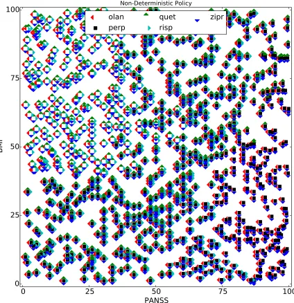
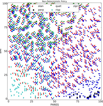
The purpose of our empirical study is to demonstrate that our non-deterministic fitted-Q algorithm is feasible to use on real clinical trial data, and that it can offer increased choice over other approaches in a real-world setting. We will discuss several plots of different NDPs. Each point on a plot represents one value of s1 in our data set, and at each point
is placed a marker for each action recommended by an NDP5. To use the plots to make
a decision for Phase 1, one would find the point on the plot corresponding to a current patient’s state, and see what actions are recommended for that state. One would then decide among them using expert knowledge, knowing that according to the data and the chosen solution concept, any of those actions would be optimal. Then the process would be repeated should the patient move on to Phase 2, using the corresponding plots for T “ 2 (not shown.) It is important to note that the axes in Figures 5 through 8 represent state, even though the same features (measured after treatment) are also used as reward values.
One can think of all of the learned NDPs that we present in the following experiments as transformations of the raw trajectory data into recommended actions, made under different solution concepts. The choice of solution concept is subjective and tied an application at
0
25
50
75
100
PANSS
0
25
50
75
100
BMI
Non-Deterministic Policy from Convex Combinations of Rewards
olan
perp
quet
risp
zipr
Figure 5: NDP produced by taking the union over actions recommended by Lizotte et al. (2010, 2012)
0
25
50
75
100
PANSS
0
25
50
75
100
BMI
Non-Deterministic Policy
olan
perp
quet
risp
zipr
Figure 6: NDP produced by ΠD
ă with Pareto Domination.
Figure 5 serves as our baseline. It shows the NDP at Phase 1 produced using the convex combination technique of Lizotte et al. (2012), which assumes a linear scalarization function (equivalent to the convex Pareto partial order) and assumes that preferences are fixed over time. One can see that for a large part of the state space, only ziprasidoneİ and olanzapineđare recommended. This occurs because for much of the state space, ziprasidoneİ
0
25
50
75
100
PANSS
0
25
50
75
100
BMI
Non-Deterministic Policy
olan
perp
quet
risp
zipr
Figure 7: CATIE NDP for Phase 1 made using ΠD
ă; “warning” actions that would have been eliminated by Practical Domination but not by Strong Practical Domination have been removed.
this NDP, the mean number of choices per state is 2.26, and 100% of states have had one or more actions eliminated.
In our opinion, the convex Pareto domination solution criterion is overly eager to elimi-nate actions in this context, and the assumption of a fixed scalarization function is unrealis-tic. Figure 6 shows the NDP learned for Phase 1 using Algorithm 1 with Pareto domination and ΠD
0
25
50
75
100
PANSS
0
25
50
75
100
BMI
Non-Deterministic Policy
olan
perp
quet
risp
zipr
Figure 8: NDP produced by Π@
ă with Strong Practical Domination.
are larger. Despite the increased choice available, a user following these recommendations can still achieve a value on the Pareto frontier even if their preferences change in Phase 2. In this NDP, the mean number of choices per state is 4.14, and 68% of states have had at least one eliminated.
than another action in order to dominate it, and although we have removed actions that were warned to have a bad trade-off—those that were slightly better for one reward but practically worse for another—we still provide increased choice over using the Pareto frontier alone. In this NDP, the mean number of choices per state is 4.30, and 55% of states have had one or more actions eliminated.
We now consider using the same solution concept but the more strict Π@
ă definition for constructing the NDP. Figure 8 shows the NDP learned for Phase 1 using our algorithm with Strong Practical Domination (∆1 “ ∆2 “ 2.5) and Π@ă. Again, an action must be practically better than another action in order to dominate it, which tends to increase action choices. However, recall that for Π@
ă we only recommend actions that are not dominated by another action for any future policy. Hence, these actions are extremely “safe” in the sense that they achieve an expected value on the ăsp-frontier as long as the user selects
from our recommended actions in the future. In this NDP, the mean number of choices per state is 2.56, and 100% of states have had one or more actions eliminated. Hence, we have a trade-off here: Relative to ΠD
ă, this approach reduces choice, yet increases safety; whether or not this is preferable will depend on the application at hand. That said, using Π@
ă in this way provides more choice than recommending actions based on convex Pareto optimality and a fixed future policy, while at the same time providing a guarantee that the recommended actions are safe choices even if preferences change.
Using φ-consistency to reduce the size of Qt was critical for all of our analyses. In the
Phase 2 Tolerability NDP there are over 10124 consistent policies but only 1213φ-consistent policies, and in the Phase 2 Efficacy NDP there are 1 048 576 consistent policies but only 98 φ-consistent policies. Finding theφ-consistent policies took less than one minute on an Intel Core i7 at 3.4 GHz using Python and CPLEX.
8. Discussion
Our overarching goal is to expand the toolbox of data analysts by developing new, useful methods for producing decision support systems in very challenging settings. To have maximum impact, decision support must appropriately take into account the sequential aspects of the problem at hand and at the same time acknowledge the fact that different decision makers have different preferences. Working toward this goal, we have presented a suite of novel ideas for learning non-deterministic policies for MDPs with multiple objectives. We gave a formulation of fitted-Q iteration for multiple basis rewards, we discussed ways of producing an NDP from a setQtofQ-functions that depend on different future policies,
we introduced the idea of φ-consistent policies to control computational complexity, and we introduced “practical domination” to help users express their preference over actions without explicitly eliciting a preference over basis rewards. Finally, we showed using clinical trial data how our method could be used, and we showed that the NDPs we are able to learn offer more optimal action choice than previous approaches.
Rather than restrict ourselves by trying to identify a single “best approach” for all decision support systems, we have developed an algorithm that is modular: One could substitute another notion of domination for the ones we proposed if another notion is more appropriate for a given problem domain. Regardless of this choice, our algorithm will suggest sets of actions that are optimal in the sense we have described. For some applications, ΠD
ă may be appropriate; for other more conservative applications Π@ă may be the only responsible choice. Note that we are not dictating how the output from the NDP is used; one could imagine an interface that accepted patient state information and displayed richer information based on ΠD
ă, Π@ă, and perhaps plots like Figure 2 to convey to the user what the pros and cons are for the different actions. Our contributions make a wide variety of new decision support systems possible.
Acknowledgments
We acknowledge support from the Natural Sciences and Engineering Research Council of Canada. Data used in the preparation of this article were obtained from the limited access data sets distributed from the NIH-supported “Clinical Antipsychotic Trials of Intervention Effectiveness in Schizophrenia” (CATIE-Sz). The study was supported by NIMH Contract N01MH90001 to the University of North Carolina at Chapel Hill. TheClinicalTrials.gov
identifier is NCT00014001. This manuscript reflects the views of the authors and may not reflect the opinions or views of the CATIE-Sz Study Investigators or the NIH.
References
O. Alagoz, H. Hsu, A. J. Schaefer, and M. S. Roberts. Markov decision processes: A tool for sequential decision making under uncertainty. Medical decision making : an international journal of the Society for Medical Decision Making, 30(4):474–483, 2010. ISSN 0272-989X.
D. B. Allison, J. L. Mentore, M. Heo, L. P. Chandler, J. C. Cappelleri, M. C. Infante, and P. J. Weiden. Antipsychotic-induced weight gain: A comprehensive research synthesis.
American Journal of Psychiatry, 156:1686–1696, November 1999.
D. P. Bertsekas. Dynamic Programming and Optimal Control, Vol. II. Athena Scientific, 3rd edition, 2007. ISBN 1886529302, 9781886529304.
D. P. Bertsekas and J. N. Tsitsiklis. Neuro-Dynamic Programming, chapter 2.1, page 12. Athena Scientific, 1996.
D. Blatt, S. A. Murphy, and J. Zhu. A-learning for approximate planning. Technical Report 04-63, The Methodology Center, Penn. State University, 2004.
E. Brunskill and S. J. Russell. Partially observable sequential decision making for problem selection in an intelligent tutoring system. In Educational Data Mining (EDM), pages 327–328, 2011.
A. Castelletti, S. Galelli, M. Restelli, and R. Soncini-Sessa. Tree-based reinforcement learn-ing for optimal water reservoir operation. Water Resources Research, 46, 2010.
K. Chatterjee, R. Majumdar, and T. Henzinger. Markov decision processes with multiple objectives. In STACS, pages 325–336, 2006.
M. Chi, K. VanLehn, D. Litman, and P. Jordan. An evaluation of pedagogical tutorial tactics for a natural language tutoring system: A reinforcement learning approach. Int. J. Artif. Intell. Ed., 21(1-2):83–113, January 2011. ISSN 1560-4292.
R. D. Cook and S. Weisberg. Applied Regression Including Computing and Graphics. Wiley, August 1999.
CPLEX. ILOG CPLEX Optimizer.
http://www-01.ibm.com/software/integration/optimization/cplex-optimizer/, 2012.
M. Ehrgott. Multicriteria Optimization, chapter 3. Springer, second edition, 2005.
D. Ernst, P. Geurts, and L. Wehenkel. Tree-Based Batch Mode Reinforcement Learning.
Journal of Machine Learning Research, 6:503–556, 2005.
T. Hastie, R. Tibshirani, and J. Friedman. The Elements of Statistical Learning. Springer Series in Statistics. Springer New York Inc., New York, NY, USA, 2001.
R. Henderson, P. Ansell, and D. Alshibani. Regret-regression for optimal dynamic treatment regimes. Biometrics, 66:1192–1201, 2010.
S. R. Kay, A. Fiszbein, and L. A. Opfer. The Positive and Negative Syndrome Scale (PANSS) for schizophrenia. Schizophrenia Bulletin, 13(2):261–276, 1987.
R. E. Kirk. Practical significance: A concept whose time has come. Educational and Psychological Measurement, 56(5):746–759, October 1996.
E. B. Laber, D. J. Lizotte, and B. Ferguson. Set-valued dynamic treatment regimes for competing outcomes. Biometrics, 70(1):53–61, 2014a.
E. B. Laber, D. J. Lizotte, M. Qian, W. E. Pelham, and S. A. Murphy. Dynamic treatment regimes: technical challenges and applications. Electronic Journal of Statistics, 8(1): 1225–1272, 2014b.
D. J. Lizotte, M. Bowling, and S. A. Murphy. Efficient reinforcement learning with multiple reward functions for randomized clinical trial analysis. In International Conference on Machine Learning (ICML), 2010.
D. J. Lizotte, M. Bowling, and S. A. Murphy. Linear fitted-Q iteration with multiple reward functions. Journal of Machine Learning Research, 13:3253–3295, Nov 2012.
K. M. Miettinen. Nonlinear Multiobjective Optimization. Kluwer, 1999.
M. Milani Fard and J. Pineau. Non-deterministic policies in Markovian decision processes.
E. E. M. Moodie, T. S. Richardson, and D. A. Stephens. Demystifying optimal dynamic treatment regimes. Biometrics, 63(2):447–455, 2007.
B. K. Natarajan. On learning sets and functions. Machine Learning, 4(1):67–97, 1989.
P. Perny and P. Weng. On finding compromise solutions in multiobjective Markov decision processes. InEuropean Conference on Artificial Intelligence (ECAI), pages 969–970, 2010.
C. P˘aduraru, D. Precup, J. Pineau, and G. Com˘anici. A study of off-policy learning in com-putational sustainability. In European Workshop on Reinforcement Learning (EWRL), volume 24 of JMLR Workshop and Conference Proceedings, pages 89–102, 2012.
A. N. Rafferty, E. Brunskill, T. L. Griffiths, and P. Shafto. Faster teaching by POMDP planning. In International Conference on Artificial Intelligence in Education (AIED), pages 280–287, Berlin, Heidelberg, 2011. Springer-Verlag. ISBN 978-3-642-21868-2.
D. M. Roijers, P. Vamplew, S. Whiteson, and R. Dazeley. A survey of multi-objective sequential decision-making. Journal of Artificial Intelligence Research, 48:67–113, 2013.
S. Shalev-Shwartz and S. Ben-David. Understanding Machine Learning. Cambridge Uni-versity Press, 2014. Cambridge Books Online.
S. Shortreed, E. B. Laber, D. J. Lizotte, T. S. Stroup, J. Pineau, and S. A. Murphy. In-forming sequential clinical decision-making through reinforcement learning: an empirical study. Machine Learning, 84(1–2):109–136, 2011.
V. J. Strecher, S. Shiffman, and R. West. Moderators and mediators of a web-based computer-tailored smoking cessation program among nicotine patch users. Nicotine & tobacco research, 8(S. 1):S95, 2006.
T. S. Stroup and al. The national institute of mental health clinical antipsychotic trials of intervention effectiveness (CATIE) project: Schizophrenia trial design and protocol development. Schizophrenia Bulletin, 29(1), 2003.
M. S. Swartz, D. O. Perkins, T. S. Stroup, J. P. McEvoy, J. M. Nieri, and D. D. Haal. Assessing clinical and functional outcomes in the clinical antipsychotic of intervention effectiveness (CATIE) schizophrenia trial. Schizophrenia Bulletin, 29(1), 2003.
I. Tsochantaridis, T. Joachims, T. Hoffmann, and Y. Altun. Large margin methods for structured and independent output variables. Journal of Machine Learning Research, 6: 1453–1484, 2005.
P. Vamplew, R. Dazeley, E. Barker, and A. Kelarev. Constructing stochastic mixture policies for episodic multiobjective reinforcement learning tasks. In The 22nd Australasian Conf. on AI, 2009.